On Benchmarking, Part 6
20 Feb 2017This is a long series of posts where I try to teach myself how to run rigorous, reproducible microbenchmarks on Linux. You may want to start from the first one and learn with me as I go along. I am certain to make mistakes, please write be back in this bug when I do.
In my previous post I chose the Mann-Whitney U
Test
to perform an statistical test of hypothesis comparing
array_based_order_book vs. map_based_order_book.
I also explored why neither the arithmetic mean, nor the median are
good measures of effect in this case.
I learned about the Hodges-Lehmann
Estimator
as a better measure of effect for performance improvement.
Finally I used some mock data to familiarize myself with these tools.
In this post I will solve the last remaining issue from my Part 1 of this series. Specifically [I12]: how can anybody reproduce the results that I obtained.
The Challenge of Reproducibility
I have gone to some length to make the tests producible:
- The code under test, and the code used to generate the results is available from my github account.
- The code includes full instructions to compile the system, and in addition to the human readable documentation there are automated scripts to compile the system.
- I have also documented which specific version of the code was used to generate each post, so a potential reader (maybe a future version of myself), can fetch the specific version and rerun the tests.
- Because compilation instructions can be stale, or incorrect, or hard to follow, I have made an effort to provide pre-packaged docker images with all the development tools and dependencies necessary to compile and execute the benchmarks.
Despite these efforts I expect that it would be difficult, if not impossible, to reproduce the results for a casual or even a persistent reader: the exact hardware and software configuration that I used, though documented, would be extremely hard to put together again. Within months the packages used to compile and link the code will no longer be current, and may even disappear from the repositories where I fetched them from. In addition, it would be quite a task to collect the specific parts to reproduce a custom-built computer put together several years ago.
I think containers may offer a practical way to package the development environment, the binaries, and the analysis tools in a form that allows us to reproduce the results easily.
I do not believe the reader would be able to reproduce the absolute performance numbers, those depend closely on the physical hardware used. But one should be able to reproduce the main results, such as the relative performance improvements, or the fact that we observed a statistically significant improvement in performance.
I aim to explore these ideas in this post, though I cannot say that I have fully solved the problems that arise when trying to use them.
Towards Reproducible Benchmarks
As part of its continuous integration builds JayBeams creates runtime images with all the necessary code to run the benchmarks. I have manually tagged the images that I used in this post, with the post name, so they can be easily fetched. Assuming you have a Linux workstation (or server), with docker configured you should be able to execute the following commands to run the benchmark:
$ TAG=2017-02-20-on-benchmarking-part-6
$ sudo docker pull coryan/jaybeams-runtime-fedora25:$TAG
$ sudo docker run --rm -i -t --cap-add sys_nice --privileged \
    --volume $PWD:/home/jaybeams --workdir /home/jaybeams \
    coryan/jaybeams-runtime-fedora25:$TAG \
    /opt/jaybeams/bin/bm_order_book_generate.sh
The results will be generated in a local file named
bm_order_book_generate.1.results.csv.
You can verify I used the same version of the runtime image with the
following command:
$ sudo docker inspect -f '{{ .Id }}' \
    coryan/jaybeams-runtime-fedora25:$TAG
sha256:641ea7fc96904f8b940afb0775d25b29fd54b8338ec7ba5aa0ce7cff77c3d0c7
Reproduce the Analysis
A separate image can be used to reproduce the analysis. I prefer a separate image because the analysis image tends to be relatively large:
$ cd $HOME
$ sudo docker pull coryan/jaybeams-analysis:$TAG
$ sudo docker inspect -f '{{ .Id }}' \
    coryan/jaybeams-analysis:$TAG
sha256:7ecdbe5950fe8021ad133ae8acbd9353484dbb3883be89d976d93557e7271173
First we copy the results produced earlier to a directory hierarchy that will work with my blogging platform:
$ cd $HOME/coryan.github.io
$ cp bm_order_book_generate.1.results.csv \
  public/2017/02/20/on-benchmarking-part-6/workstation-results.csv
$ sudo docker run --rm -i -t --volume $PWD:/home/jaybeams \
    --workdir /home/jaybeams coryan/jaybeams-analysis:$TAG \
    /opt/jaybeams/bin/bm_order_book_analyze.R \
    public/2017/02/20/on-benchmarking-part-6/workstation-results.csv \
    public/2017/02/20/on-benchmarking-part-6/workstation/ \
    _includes/2017/02/20/on-benchmarking-part-6/workstation-report.md
The resulting report is included later in this post.
Running on Public Cloud Virtual Machines
Though the previous steps have addressed the problems with recreating the software stack used to run the benchmarks I have not addressed the problem of reproducing the hardware stack.
I thought I could solve this problem using public cloud, such as Amazon Web Services, or Google Cloud Platform. Unfortunately I do not know (yet?) how to control the environment on a public cloud virtual machine to avoid auto-correlation in the sample data.
Below I will document the steps to run the benchmark on a virtual machine, but I should warn the reader upfront that the results are suspect.
The resulting report is included later in this post.
Create the Virtual Machine
I have chosen Google’s public cloud simply because I am more familiar with it, I make no claims as to whether it is better or worse than the alternatives.
# Set these environment variables based on your preferences
# for Google Cloud Platform
$ PROJECT=[your project name here]
$ ZONE=[your favorite zone here]
$ PROJECTID=$(gcloud projects --quiet list | grep $PROJECT | \
    awk '{print $3}')

# Create a virtual machine to run the benchmark
$ VM=benchmark-runner
$ gcloud compute --project $PROJECT instances \
  create $VM \
  --zone $ZONE --machine-type "n1-standard-2" --subnet "default" \
  --maintenance-policy "MIGRATE" \
  --scopes "https://www.googleapis.com/auth/cloud-platform" \
  --service-account \
    ${PROJECTID}-compute@developer.gserviceaccount.com \
  --image "ubuntu-1604-xenial-v20170202" \
  --image-project "ubuntu-os-cloud" \
  --boot-disk-size "32" --boot-disk-type "pd-standard" \
  --boot-disk-device-name $VM
Login and Run the Benchmark
$ gcloud compute --project $PROJECT ssh \
  --ssh-flag=-A --zone $ZONE $VM
$ sudo apt-get update && sudo apt-get install -y docker.io
$ TAG=2017-02-20-on-benchmarking-part-6
$ sudo docker run --rm -i -t --cap-add sys_nice --privileged \
    --volume $PWD:/home/jaybeams --workdir /home/jaybeams \
    coryan/jaybeams-runtime-ubuntu16.04:$TAG \
    /opt/jaybeams/bin/bm_order_book_generate.sh 100000
$ sudo docker inspect -f '{{ .Id }}' \
    coryan/jaybeams-runtime-ubuntu16.04:$TAG
sha256:c70b9d2d420bd18680828b435e8c39736e902b830426c27b4cf5ec32243438e4
$ exit
Fetch the Results and Generate the Reports
# Back in your workstation ...
$ cd $HOME/coryan.github.io
$ gcloud compute --project $PROJECT copy-files --zone $ZONE \
  $VM:bm_order_book_generate.1.results.csv \
  public/2017/02/20/on-benchmarking-part-6/vm-results.csv
$ TAG=2017-02-20-on-benchmarking-part-6
$ sudo docker run --rm -i -t --volume $PWD:/home/jaybeams \
    --workdir /home/jaybeams coryan/jaybeams-analysis:$TAG \
    /opt/jaybeams/bin/bm_order_book_analyze.R \
    public/2017/02/20/on-benchmarking-part-6/vm-results.csv \
    public/2017/02/20/on-benchmarking-part-6/vm/ \
    _includes/2017/02/20/on-benchmarking-part-6/vm-report.md
Cleanup
# Delete the virtual machine
$ gcloud compute --project $PROJECT \
    instances delete $VM --zone $ZONE
Docker Image Creation
All that remains at this point is to describe how the images
themselves are created.
I automated the process to create images as part of the continuous
integration builds for JayBeams.
After each commit to the master
branch travis checks out the
code, uses an existing development environment to compile and test the
code, and then creates the runtime and analysis images.
If the runtime and analysis images differ from the existing images in the github repository the new images are automatically pushed to the github repository.
If necessary, a new development image is also created as part of the continuous integration build. This means that the development image might be one build behind, as the latest runtime and analysis images may have been created with a previous build image. I have an outstanding bug to fix this problem. In practice this is not a major issue because the development environment changes rarely.
An appendix to this post includes step-by-step instructions on what the automated continuous integration build does.
Tagging Images for Final Report
The only additional step is to tag the images used to create this report, so they are not lost in the midst of time:
$ TAG=2017-02-20-on-benchmarking-part-6
$ for image in \
    coryan/jaybeams-analysis \
    coryan/jaybeams-runtime-fedora25 \
    coryan/jaybeams-runtime-ubuntu16.04; do
  sudo docker pull ${image}:latest
  sudo docker tag ${image}:latest ${image}:$TAG
  sudo docker push ${image}:$TAG
done
Summary
In this post I addressed the last remaining issue identified at the beginning of this series. I have made the tests as reproducible as I know how. A reader can execute the tests in a public cloud server, or if they prefer on their own Linux workstation, by downloading and executing pre-compiled images.
It is impossible to predict for how long those images will remain usable, but they certainly go a long way to make the tests and analysis completely scripted.
Furthermore, the code to create the images themselves has been fully automated.
Next Up
I will be taking a break from posting about benchmarks and statistics, I want to go back to writing some code, more than talking about how to measure code.
Notes
All the code for this post is available from the
78bdecd855aa9c25ce606cbe2f4ddaead35706f1
version of JayBeams, including the Dockerfiles used to create the
images.
The images themselves were automatically created using travis.org, a service for continuous integration. The travis configuration file and helper script are also part of the code for JayBeams.
The data used generated and used in this post is also available: workstation-results.csv, and vm-results.csv.
Metadata about the tests, including platform details can be found in comments embedded with the data files.
Appendix: Manual Image Creation
Normally the images are created by an automated build, but for completeness we document the steps to create one of the runtime images here. We assume the system has been configured to run docker, and the desired version of JayBeams has been checked out in the current directory.
First we create a virtual machine, that guarantees that we do not have hidden dependencies on previously installed tools or configurations:
$ VM=jaybeams-build
$ gcloud compute --project $PROJECT instances \
  create $VM \
  --zone $ZONE --machine-type "n1-standard-2" --subnet "default" \
  --maintenance-policy "MIGRATE" \
  --scopes "https://www.googleapis.com/auth/cloud-platform" \
  --service-account \
    ${PROJECTID}-compute@developer.gserviceaccount.com \
  --image "ubuntu-1604-xenial-v20170202" \
  --image-project "ubuntu-os-cloud" \
  --boot-disk-size "32" --boot-disk-type "pd-standard" \
  --boot-disk-device-name $VM
Then we connect to the virtual machine:
$ gcloud compute --project $PROJECT ssh \
  --ssh-flag=-A --zone $ZONE $VM
install the latest version of docker on the virtual machine:
# ... these commands are on the virtual machine ..
$ curl -fsSL https://apt.dockerproject.org/gpg | \
    sudo apt-key add -
$ sudo add-apt-repository \
       "deb https://apt.dockerproject.org/repo/ \
       ubuntu-$(lsb_release -cs) \
       main"
$ sudo apt-get update && sudo apt-get install -y docker-engine
we set the build parameters:
$ export IMAGE=coryan/jaybeamsdev-ubuntu16.04 \
    COMPILER=g++ \
    CXXFLAGS=-O3 \
    CONFIGUREFLAGS="" \
    CREATE_BUILD_IMAGE=yes \
    CREATE_RUNTIME_IMAGE=yes \
    CREATE_ANALYSIS_IMAGE=yes \
    TRAVIS_BRANCH=master \
    TRAVIS_PULL_REQUEST=false
Checkout the code:
$ git clone https://github.com/coryan/jaybeams.git
$ cd jaybeams
$ git checkout 78bdecd855aa9c25ce606cbe2f4ddaead35706f1
Download the build image and compile, test, and install the code in a staging area:
$ sudo docker pull ${IMAGE?}
$ sudo docker run --rm -it \
    --env CONFIGUREFLAGS=${CONFIGUREFLAGS} \
    --env CXX=${COMPILER?} \
    --env CXXFLAGS="${CXXFLAGS}" \
    --volume $PWD:$PWD \
    --workdir $PWD \
    ${IMAGE?} ci/build-in-docker.sh
To recreate the runtime image locally, this will not push to the github repository, because the github credentials are not provided:
$ ci/create-runtime-image.sh
Likewise we can recreate the analysis image:
$ ci/create-analysis-image.sh
We can examine the images created so far:
$ sudo docker images
Before we exit and delete the virtual machine:
$ exit

# ... back on your workstation ...
$ gcloud compute --project $PROJECT \
    instances delete $VM --zone $ZONE
Report for workstation-results.csv
We load the file, which has a well-known name, into a data.frame
structure:
data <- read.csv(
    file=data.filename, header=FALSE, comment.char='#',
    col.names=c('book_type', 'nanoseconds'))
The raw data is in nanoseconds, I prefer microseconds because they are easier to think about:
data$microseconds <- data$nanoseconds / 1000.0We also annotate the data with a sequence number, so we can plot the sequence of values:
data$idx <- ave(
    data$microseconds, data$book_type, FUN=seq_along)
At this point I am curious as to how the data looks like, and probably you too, first just the usual summary:
data.summary <- aggregate(
    microseconds ~ book_type, data=data, FUN=summary)
kable(cbind(
    as.character(data.summary$book_type),
data.summary$microseconds))| Min. | 1st Qu. | Median | Mean | 3rd Qu. | Max. | |
|---|---|---|---|---|---|---|
| array | 223 | 310 | 398 | 454 | 541 | 1550 |
| map | 718 | 1110 | 1190 | 1190 | 1270 | 1960 |
Then we visualize the density functions, if the data had extreme tails or other artifacts we would rejects it:
ggplot(data=data, aes(x=microseconds, color=book_type)) +
    theme(legend.position="bottom") +
    facet_grid(book_type ~ .) + stat_density()
We also examine the boxplots of the data:
ggplot(data=data,
       aes(y=microseconds, x=book_type, color=book_type)) +
    theme(legend.position="bottom") + geom_boxplot()
Check Assumptions: Validate the Data is Independent
I inspect the data in case there are obvious problems with independence of the samples. Output as PNG files. While SVG files look better in a web page, large SVG files tend to crash browsers.
ggplot(data=data,
       aes(x=idx, y=microseconds, color=book_type)) +
    theme(legend.position="bottom") +
    facet_grid(book_type ~ .) + geom_point()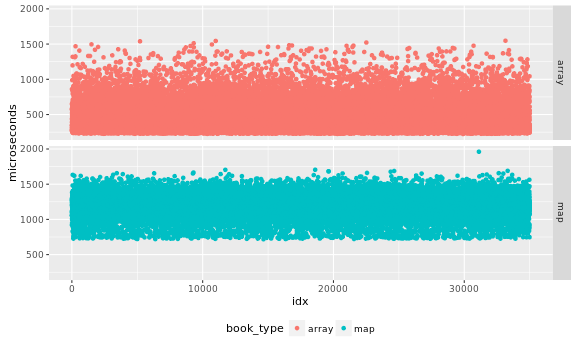
I would like an analytical test to validate the samples are indepedent, a visual inspection of the data may help me detect obvious problems, but I may miss more subtle issues. For this part of the analysis it is easier to separate the data by book type, so we create two timeseries for them:
data.array.ts <- ts(
    subset(data, book_type == 'array')$microseconds)
data.map.ts <- ts(
    subset(data, book_type == 'map')$microseconds)
Plot the correlograms:
acf(data.array.ts)
acf(data.map.ts)
Compute the maximum auto-correlation factor, ignore the first value, because it is the auto-correlation at lag 0, which is always 1.0:
max.acf.array <- max(abs(
    tail(acf(data.array.ts, plot=FALSE)$acf, -1)))
max.acf.map <- max(abs(
    tail(acf(data.map.ts, plot=FALSE)$acf, -1)))
I think any value higher than indicates that the samples are not truly independent:
max.autocorrelation <- 0.05
if (max.acf.array >= max.autocorrelation |
    max.acf.map >= max.autocorrelation) {
    warning("Some evidence of auto-correlation in ",
         "the samples max.acf.array=",
         round(max.acf.array, 4),
         ", max.acf.map=",
         round(max.acf.map, 4))
} else {
    cat("PASSED: the samples do not exhibit high auto-correlation")
}
## PASSED: the samples do not exhibit high auto-correlationI am going to proceed, even though the data on virtual machines tends to have high auto-correlation.
Power Analysis: Estimate Standard Deviation
Use bootstraping to estimate the standard deviation, we are going to need a function to execute in the bootstrapping procedure:
sd.estimator <- function(D,i) {
    return(sd(D[i,'microseconds']));
}
Because this can be slow, we use all available cores:
core.count <- detectCores()
b.array <- boot(
    data=subset(data, book_type == 'array'), R=10000,
    statistic=sd.estimator,
    parallel="multicore", ncpus=core.count)
plot(b.array)
ci.array <- boot.ci(
    b.array, type=c('perc', 'norm', 'basic'))

b.map <- boot(
    data=subset(data, book_type == 'map'), R=10000,
    statistic=sd.estimator,
    parallel="multicore", ncpus=core.count)
plot(b.map)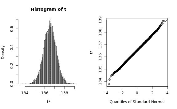
ci.map <- boot.ci(
    b.map, type=c('perc', 'norm', 'basic'))
We need to verify that the estimated statistic roughly follows a normal distribution, otherwise the bootstrapping procedure would require a lot more memory than we have available: The Q-Q plots look reasonable, so we can estimate the standard deviation using a simple procedure:
estimated.sd <- ceiling(max(
    ci.map$percent[[4]], ci.array$percent[[4]],
    ci.map$basic[[4]], ci.array$basic[[4]],
    ci.map$normal[[3]], ci.array$normal[[3]]))
cat(estimated.sd)
## 197Power Analysis: Determine Required Number of Samples
We need to determine if the sample size was large enough given the estimated standard deviation, the expected effect size, and the statistical test we are planning to use.
The is the minimum effect size that we could be interested in is based on saving at least one cycle per operation in the classes we are measuring.
The test executes 20,000 iterations:
test.iterations <- 20000and we assume that the clock cycle is approximately 3Ghz:
clock.ghz <- 3We can use this to compute the minimum interesting effect:
min.delta <- 1.0 / (clock.ghz * 1000.0) * test.iterations
cat(min.delta)
## 6.667That is, any result smaller than 6.6667 microseconds would not be interesting and should be rejected. We need a few more details to compute the minimum number of samples, first, the desired significance of any results, which we set to:
desired.significance <- 0.01Then, the desired statistical power of the test, which we set to:
desired.power <- 0.95We are going to use a non-parametric test, which has a 15% overhead above the t-test:
nonparametric.extra.cost <- 1.15In any case, we will require at least 5000 iterations, because it is relatively fast to run that many:
min.samples <- 5000If we do not have enough power to detect 10 times the minimum effect we abort the analysis, while if we do not have enough samples to detect the minimum effect we simply generate warnings:
required.pwr.object <- power.t.test(
    delta=10 * min.delta, sd=estimated.sd,
    sig.level=desired.significance, power=desired.power)
print(required.pwr.object)
##
## Two-sample t test power calculation
##
## n = 312.8
## delta = 66.67
## sd = 197
## sig.level = 0.01
## power = 0.95
## alternative = two.sided
##
## NOTE: n is number in *each* groupWe are going to round the number of iterations to the next higher multiple of 1000, because it is easier to type, say, and reason about nice round numbers:
required.nsamples <- max(
    min.samples, 1000 * ceiling(nonparametric.extra.cost *
                                required.pwr.object$n / 1000))
cat(required.nsamples)
## 5000That is, we need 5000 samples to detect an effect of 66.67 microseconds at the desired significance and power levels.
if (required.nsamples > length(data.array.ts)) {
    stop("Not enough samples in 'array' data to",
         " detect expected effect (",
         10 * min.delta,
         ") should be >=", required.nsamples,
         " actual=", length(array.map.ts))
}
if (required.nsamples > length(data.map.ts)) {
    stop("Not enough samples in 'map' data to",
         " detect expected effect (",
         10 * min.delta,
         ") should be >=", required.nsamples,
         " actual=", length(map.map.ts))
}
desired.pwr.object <- power.t.test(
delta=min.delta, sd=estimated.sd,
sig.level=desired.significance, power=desired.power)
desired.nsamples <- max(
min.samples, 1000 * ceiling(nonparametric.extra.cost *
desired.pwr.object$n / 1000))
print(desired.pwr.object)##
## Two-sample t test power calculation
##
## n = 31112
## delta = 6.667
## sd = 197
## sig.level = 0.01
## power = 0.95
## alternative = two.sided
##
## NOTE: n is number in *each* groupThat is, we need at least 36000 samples to detect the minimum interesting effect of 6.6667 microseconds. Notice that our tests have 35000 samples.
if (desired.nsamples > length(data.array.ts) |
    desired.nsamples > length(data.map.ts)) {
    warning("Not enough samples in the data to",
            " detect the minimum interating effect (",
            round(min.delta, 2), ") should be >= ",
            desired.nsamples,
            " map-actual=", length(data.map.ts),
            " array-actual=", length(data.array.ts))
} else {
    cat("PASSED: The samples have the minimum required power")
}
## Warning: Not enough samples in the data to detect the
## minimum interating effect (6.67) should be >= 36000 map-
## actual=35000 array-actual=35000Run the Statistical Test
We are going to use the Mann-Whitney U test to analyze the results:
data.mw <- wilcox.test(
    microseconds ~ book_type, data=data, conf.int=TRUE)
estimated.delta <- data.mw$estimate
The estimated effect is -771.5501 microseconds, if this number is too small we need to stop the analysis:
if (abs(estimated.delta) < min.delta) {
    stop("The estimated effect is too small to",
         " draw any conclusions.",
         " Estimated effect=", estimated.delta,
         " minimum effect=", min.delta)
} else {
    cat("PASSED: the estimated effect (",
        round(estimated.delta, 2),
        ") is large enough.")
}
## PASSED: the estimated effect ( -771.5 ) is large enough.Finally, the p-value determines if we can reject the null hypothesis
at the desired significance.
In our case, failure to reject means that we do not have enough
evidence to assert that the array_based_order_book is faster or
slower than map_based_order_book.
If we do reject the null hypothesis then we can use the
Hodges-Lehmann estimator
to size the difference in performance,
aka the effect of our code changes.
if (data.mw$p.value >= desired.significance) {
    cat("The test p-value (", round(data.mw$p.value, 4),
        ") is larger than the desired\n",
        "significance level of alpha=",
        round(desired.significance, 4), "\n", sep="")
    cat("Therefore we CANNOT REJECT the null hypothesis",
        " that both the 'array'\n",
        "and 'map' based order books have the same",
        " performance.\n", sep="")
} else {
    interval <- paste0(
        round(data.mw$conf.int, 2), collapse=',')
    cat("The test p-value (", round(data.mw$p.value, 4),
        ") is smaller than the desired\n",
        "significance level of alpha=",
        round(desired.significance, 4), "\n", sep="")
    cat("Therefore we REJECT the null hypothesis that",
        " both the\n",
        " 'array' and 'map' based order books have\n",
        "the same performance.\n", sep="")
    cat("The effect is quantified using the Hodges-Lehmann\n",
        "estimator, which is compatible with the\n",
        "Mann-Whitney U test, the estimator value\n",
        "is ", round(data.mw$estimate, 2),
        " microseconds with a 95% confidence\n",
        "interval of [", interval, "]\n", sep="")
}
## The test p-value (0) is smaller than the desired
## significance level of alpha=0.01
## Therefore we REJECT the null hypothesis that both the
## 'array' and 'map' based order books have
## the same performance.
## The effect is quantified using the Hodges-Lehmann
## estimator, which is compatible with the
## Mann-Whitney U test, the estimator value
## is -771.5 microseconds with a 95% confidence
## interval of [-773.77,-769.32]Mini-Colophon
This report was generated using knitr
the details of the R environment are:
library(devtools)
devtools::session_info()
## Session info -----------------------------------------------## setting value
## version R version 3.2.3 (2015-12-10)
## system x86_64, linux-gnu
## ui X11
## language (EN)
## collate C
## tz Zulu
## date 2017-02-20## Packages ---------------------------------------------------## package * version date source
## Rcpp 0.12.3 2016-01-10 CRAN (R 3.2.3)
## boot * 1.3-17 2015-06-29 CRAN (R 3.2.1)
## colorspace 1.2-4 2013-09-30 CRAN (R 3.1.0)
## devtools * 1.12.0 2016-12-05 CRAN (R 3.2.3)
## digest 0.6.9 2016-01-08 CRAN (R 3.2.3)
## evaluate 0.10 2016-10-11 CRAN (R 3.2.3)
## ggplot2 * 2.0.0 2015-12-18 CRAN (R 3.2.3)
## gtable 0.1.2 2012-12-05 CRAN (R 3.0.0)
## highr 0.6 2016-05-09 CRAN (R 3.2.3)
## httpuv 1.3.3 2015-08-04 CRAN (R 3.2.3)
## knitr * 1.15.1 2016-11-22 CRAN (R 3.2.3)
## labeling 0.3 2014-08-23 CRAN (R 3.1.1)
## magrittr 1.5 2014-11-22 CRAN (R 3.2.1)
## memoise 1.0.0 2016-01-29 CRAN (R 3.2.3)
## munsell 0.4.2 2013-07-11 CRAN (R 3.0.2)
## plyr 1.8.3 2015-06-12 CRAN (R 3.2.1)
## pwr * 1.2-0 2016-08-24 CRAN (R 3.2.3)
## reshape2 1.4 2014-04-23 CRAN (R 3.1.0)
## scales 0.3.0 2015-08-25 CRAN (R 3.2.3)
## servr 0.5 2016-12-10 CRAN (R 3.2.3)
## stringi 1.0-1 2015-10-22 CRAN (R 3.2.2)
## stringr 1.0.0 2015-04-30 CRAN (R 3.2.2)
## withr 1.0.2 2016-06-20 CRAN (R 3.2.3)Report for vm-results.csv
We load the file, which has a well-known name, into a data.frame
structure:
data <- read.csv(
    file=data.filename, header=FALSE, comment.char='#',
    col.names=c('book_type', 'nanoseconds'))
The raw data is in nanoseconds, I prefer microseconds because they are easier to think about:
data$microseconds <- data$nanoseconds / 1000.0We also annotate the data with a sequence number, so we can plot the sequence of values:
data$idx <- ave(
    data$microseconds, data$book_type, FUN=seq_along)
At this point I am curious as to how the data looks like, and probably you too, first just the usual summary:
data.summary <- aggregate(
    microseconds ~ book_type, data=data, FUN=summary)
kable(cbind(
    as.character(data.summary$book_type),
data.summary$microseconds))| Min. | 1st Qu. | Median | Mean | 3rd Qu. | Max. | |
|---|---|---|---|---|---|---|
| array | 237 | 327 | 407 | 456 | 529 | 15400 |
| map | 637 | 890 | 1020 | 1080 | 1220 | 17700 |
Then we visualize the density functions, if the data had extreme tails or other artifacts we would rejects it:
ggplot(data=data, aes(x=microseconds, color=book_type)) +
    theme(legend.position="bottom") +
    facet_grid(book_type ~ .) + stat_density()
We also examine the boxplots of the data:
ggplot(data=data,
       aes(y=microseconds, x=book_type, color=book_type)) +
    theme(legend.position="bottom") + geom_boxplot()
Check Assumptions: Validate the Data is Independent
I inspect the data in case there are obvious problems with independence of the samples. Output as PNG files. While SVG files look better in a web page, large SVG files tend to crash browsers.
ggplot(data=data,
       aes(x=idx, y=microseconds, color=book_type)) +
    theme(legend.position="bottom") +
    facet_grid(book_type ~ .) + geom_point()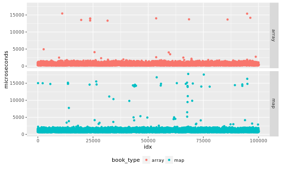
I would like an analytical test to validate the samples are indepedent, a visual inspection of the data may help me detect obvious problems, but I may miss more subtle issues. For this part of the analysis it is easier to separate the data by book type, so we create two timeseries for them:
data.array.ts <- ts(
    subset(data, book_type == 'array')$microseconds)
data.map.ts <- ts(
    subset(data, book_type == 'map')$microseconds)
Plot the correlograms:
acf(data.array.ts)
acf(data.map.ts)
Compute the maximum auto-correlation factor, ignore the first value, because it is the auto-correlation at lag 0, which is always 1.0:
max.acf.array <- max(abs(
    tail(acf(data.array.ts, plot=FALSE)$acf, -1)))
max.acf.map <- max(abs(
    tail(acf(data.map.ts, plot=FALSE)$acf, -1)))
I think any value higher than indicates that the samples are not truly independent:
max.autocorrelation <- 0.05
if (max.acf.array >= max.autocorrelation |
    max.acf.map >= max.autocorrelation) {
    warning("Some evidence of auto-correlation in ",
         "the samples max.acf.array=",
         round(max.acf.array, 4),
         ", max.acf.map=",
         round(max.acf.map, 4))
} else {
    cat("PASSED: the samples do not exhibit high auto-correlation")
}
## Warning: Some evidence of auto-correlation in the samples
## max.acf.array=0.0964, max.acf.map=0.256I am going to proceed, even though the data on virtual machines tends to have high auto-correlation.
Power Analysis: Estimate Standard Deviation
Use bootstraping to estimate the standard deviation, we are going to need a function to execute in the bootstrapping procedure:
sd.estimator <- function(D,i) {
    return(sd(D[i,'microseconds']));
}
Because this can be slow, we use all available cores:
core.count <- detectCores()
b.array <- boot(
    data=subset(data, book_type == 'array'), R=10000,
    statistic=sd.estimator,
    parallel="multicore", ncpus=core.count)
plot(b.array)
ci.array <- boot.ci(
    b.array, type=c('perc', 'norm', 'basic'))

b.map <- boot(
    data=subset(data, book_type == 'map'), R=10000,
    statistic=sd.estimator,
    parallel="multicore", ncpus=core.count)
plot(b.map)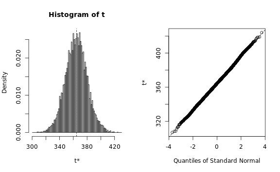
ci.map <- boot.ci(
    b.map, type=c('perc', 'norm', 'basic'))
We need to verify that the estimated statistic roughly follows a normal distribution, otherwise the bootstrapping procedure would require a lot more memory than we have available: The Q-Q plots look reasonable, so we can estimate the standard deviation using a simple procedure:
estimated.sd <- ceiling(max(
    ci.map$percent[[4]], ci.array$percent[[4]],
    ci.map$basic[[4]], ci.array$basic[[4]],
    ci.map$normal[[3]], ci.array$normal[[3]]))
cat(estimated.sd)
## 396Power Analysis: Determine Required Number of Samples
We need to determine if the sample size was large enough given the estimated standard deviation, the expected effect size, and the statistical test we are planning to use.
The is the minimum effect size that we could be interested in is based on saving at least one cycle per operation in the classes we are measuring.
The test executes 20,000 iterations:
test.iterations <- 20000and we assume that the clock cycle is approximately 3Ghz:
clock.ghz <- 3We can use this to compute the minimum interesting effect:
min.delta <- 1.0 / (clock.ghz * 1000.0) * test.iterations
cat(min.delta)
## 6.667That is, any result smaller than 6.6667 microseconds would not be interesting and should be rejected. We need a few more details to compute the minimum number of samples, first, the desired significance of any results, which we set to:
desired.significance <- 0.01Then, the desired statistical power of the test, which we set to:
desired.power <- 0.95We are going to use a non-parametric test, which has a 15% overhead above the t-test:
nonparametric.extra.cost <- 1.15In any case, we will require at least 5000 iterations, because it is relatively fast to run that many:
min.samples <- 5000If we do not have enough power to detect 10 times the minimum effect we abort the analysis, while if we do not have enough samples to detect the minimum effect we simply generate warnings:
required.pwr.object <- power.t.test(
    delta=10 * min.delta, sd=estimated.sd,
    sig.level=desired.significance, power=desired.power)
print(required.pwr.object)
##
## Two-sample t test power calculation
##
## n = 1259
## delta = 66.67
## sd = 396
## sig.level = 0.01
## power = 0.95
## alternative = two.sided
##
## NOTE: n is number in *each* groupWe are going to round the number of iterations to the next higher multiple of 1000, because it is easier to type, say, and reason about nice round numbers:
required.nsamples <- max(
    min.samples, 1000 * ceiling(nonparametric.extra.cost *
                                required.pwr.object$n / 1000))
cat(required.nsamples)
## 5000That is, we need 5000 samples to detect an effect of 66.67 microseconds at the desired significance and power levels.
if (required.nsamples > length(data.array.ts)) {
    stop("Not enough samples in 'array' data to",
         " detect expected effect (",
         10 * min.delta,
         ") should be >=", required.nsamples,
         " actual=", length(array.map.ts))
}
if (required.nsamples > length(data.map.ts)) {
    stop("Not enough samples in 'map' data to",
         " detect expected effect (",
         10 * min.delta,
         ") should be >=", required.nsamples,
         " actual=", length(map.map.ts))
}
desired.pwr.object <- power.t.test(
delta=min.delta, sd=estimated.sd,
sig.level=desired.significance, power=desired.power)
desired.nsamples <- max(
min.samples, 1000 * ceiling(nonparametric.extra.cost *
desired.pwr.object$n / 1000))
print(desired.pwr.object)##
## Two-sample t test power calculation
##
## n = 125711
## delta = 6.667
## sd = 396
## sig.level = 0.01
## power = 0.95
## alternative = two.sided
##
## NOTE: n is number in *each* groupThat is, we need at least 145000 samples to detect the minimum interesting effect of 6.6667 microseconds. Notice that our tests have 100000 samples.
if (desired.nsamples > length(data.array.ts) |
    desired.nsamples > length(data.map.ts)) {
    warning("Not enough samples in the data to",
            " detect the minimum interating effect (",
            round(min.delta, 2), ") should be >= ",
            desired.nsamples,
            " map-actual=", length(data.map.ts),
            " array-actual=", length(data.array.ts))
} else {
    cat("PASSED: The samples have the minimum required power")
}
## Warning: Not enough samples in the data to detect the
## minimum interating effect (6.67) should be >= 145000 map-
## actual=100000 array-actual=100000Run the Statistical Test
We are going to use the Mann-Whitney U test to analyze the results:
data.mw <- wilcox.test(
    microseconds ~ book_type, data=data, conf.int=TRUE)
estimated.delta <- data.mw$estimate
The estimated effect is -600.7931 microseconds, if this number is too small we need to stop the analysis:
if (abs(estimated.delta) < min.delta) {
    stop("The estimated effect is too small to",
         " draw any conclusions.",
         " Estimated effect=", estimated.delta,
         " minimum effect=", min.delta)
} else {
    cat("PASSED: the estimated effect (",
        round(estimated.delta, 2),
        ") is large enough.")
}
## PASSED: the estimated effect ( -600.8 ) is large enough.Finally, the p-value determines if we can reject the null hypothesis
at the desired significance.
In our case, failure to reject means that we do not have enough
evidence to assert that the array_based_order_book is faster or
slower than map_based_order_book.
If we do reject the null hypothesis then we can use the
Hodges-Lehmann estimator
to size the difference in performance,
aka the effect of our code changes.
if (data.mw$p.value >= desired.significance) {
    cat("The test p-value (", round(data.mw$p.value, 4),
        ") is larger than the desired\n",
        "significance level of alpha=",
        round(desired.significance, 4), "\n", sep="")
    cat("Therefore we CANNOT REJECT the null hypothesis",
        " that both the 'array'\n",
        "and 'map' based order books have the same",
        " performance.\n", sep="")
} else {
    interval <- paste0(
        round(data.mw$conf.int, 2), collapse=',')
    cat("The test p-value (", round(data.mw$p.value, 4),
        ") is smaller than the desired\n",
        "significance level of alpha=",
        round(desired.significance, 4), "\n", sep="")
    cat("Therefore we REJECT the null hypothesis that",
        " both the\n",
        " 'array' and 'map' based order books have\n",
        "the same performance.\n", sep="")
    cat("The effect is quantified using the Hodges-Lehmann\n",
        "estimator, which is compatible with the\n",
        "Mann-Whitney U test, the estimator value\n",
        "is ", round(data.mw$estimate, 2),
        " microseconds with a 95% confidence\n",
        "interval of [", interval, "]\n", sep="")
}
## The test p-value (0) is smaller than the desired
## significance level of alpha=0.01
## Therefore we REJECT the null hypothesis that both the
## 'array' and 'map' based order books have
## the same performance.
## The effect is quantified using the Hodges-Lehmann
## estimator, which is compatible with the
## Mann-Whitney U test, the estimator value
## is -600.8 microseconds with a 95% confidence
## interval of [-602.48,-599.11]Mini-Colophon
This report was generated using knitr
the details of the R environment are:
library(devtools)
devtools::session_info()
## Session info -----------------------------------------------## setting value
## version R version 3.2.3 (2015-12-10)
## system x86_64, linux-gnu
## ui X11
## language (EN)
## collate C
## tz Zulu
## date 2017-02-20## Packages ---------------------------------------------------## package * version date source
## Rcpp 0.12.3 2016-01-10 CRAN (R 3.2.3)
## boot * 1.3-17 2015-06-29 CRAN (R 3.2.1)
## colorspace 1.2-4 2013-09-30 CRAN (R 3.1.0)
## devtools * 1.12.0 2016-12-05 CRAN (R 3.2.3)
## digest 0.6.9 2016-01-08 CRAN (R 3.2.3)
## evaluate 0.10 2016-10-11 CRAN (R 3.2.3)
## ggplot2 * 2.0.0 2015-12-18 CRAN (R 3.2.3)
## gtable 0.1.2 2012-12-05 CRAN (R 3.0.0)
## highr 0.6 2016-05-09 CRAN (R 3.2.3)
## httpuv 1.3.3 2015-08-04 CRAN (R 3.2.3)
## knitr * 1.15.1 2016-11-22 CRAN (R 3.2.3)
## labeling 0.3 2014-08-23 CRAN (R 3.1.1)
## magrittr 1.5 2014-11-22 CRAN (R 3.2.1)
## memoise 1.0.0 2016-01-29 CRAN (R 3.2.3)
## munsell 0.4.2 2013-07-11 CRAN (R 3.0.2)
## plyr 1.8.3 2015-06-12 CRAN (R 3.2.1)
## pwr * 1.2-0 2016-08-24 CRAN (R 3.2.3)
## reshape2 1.4 2014-04-23 CRAN (R 3.1.0)
## scales 0.3.0 2015-08-25 CRAN (R 3.2.3)
## servr 0.5 2016-12-10 CRAN (R 3.2.3)
## stringi 1.0-1 2015-10-22 CRAN (R 3.2.2)
## stringr 1.0.0 2015-04-30 CRAN (R 3.2.2)
## withr 1.0.2 2016-06-20 CRAN (R 3.2.3)