On Benchmarking, Part 4
16 Jan 2017This is a long series of posts where I try to teach myself how to run rigorous, reproducible microbenchmarks on Linux. You may want to start from the first one and learn with me as I go along. I am certain to make mistakes, please write be back in this bug when I do.
In my previous post I framed the
performance evaluation of array_based_order_book_side<> vs.
map_based_order_book_side<> as a statistical hypothesis testing problem.
I defined the minimum effect that would of interest, operationalized
the notion of “performance”, and defined the population of interest.
I think the process of formally framing the performance evaluation can
be applied to any CPU-bound algorithm or data structure,
and it can yield interesting observations.
For example, as I wrote down the population and problem statement it became apparent that I had designed the benchmark improperly. It was not sampling a large enough population of inputs, or at least it was cumbersome to use it to generate a large sample like this. In this post I review an improved version of the benchmark, and do some exploratory data analysis to prepare for our formal data capture.
Updates
I found a bug in the driver script for the benchmark, and updated the results after fixing the bug. None of the main conclusions changed, the tests simply got more consistent, with lower standard deviation.
The New Benchmark
I implemented three changes to the benchmark, first I modified the program to generate a new input sequence on each iteration. Then I modified the program to randomly select which side of the book the iteration was going to test. Finally, I modified the benchmark to pick the first order at random as opposed to use convenient but hard-coded values.
To modify the input data on each iteration I just added
iteration_setup() and iteration_teardown() member functions to the
benchmarking fixture.
With a little extra programming
fun
I modified the
microbenchmark framework to only call those functions if they are
present.
Modifying the benchmark created a bit of programming fun. The code uses static polymorphism to represent buy vs. sell sides of the book, and I wanted to randomly select one vs. the other. With a bit of type erasure the task is completed.
Biases in the Data Collection
I paid more attention to the seeding of my PRNG, because I do not want to introduce biases in the sampling. While this is a obvious improvement this got me thinking about any other biases in the sampling.
I think there might be problems with bias, but that needs some detailed explanation of the procedure. I think the code speaks better than I could, so I refer the reader to it. The TL;DR; version for those who would rather not read code: I generate a sequence of operations incrementally. To create a new operation pick a price level based on the distribution of event depths I measured for real data, just make sure the operation is a legal change to the book. Keep track of the book implied by all these operations. At the end verify the distribution passes the criteria I set earlier in this series (p99.9 within a given range), regenerate the series from scratch if it fails the test.
Characterizing if this is a bias sampler or not would be an extremely difficult problem to tackle, for example, the probability of seeing any particular sequence of operations in the wild is unknown, beyond the characterization of the event depth distribution I found earlier. Nor do I have a good characterization of the quantities. I think the major problem is that the sequences generated by the code tend to meet the event depth distribution at every length, while the sequences in the wild may converge only slowly to the observed distribution of event depths.
This is arguably a severe pitfall in the analysis. Effectively it limits the results to “for the population of inputs that can be reached by the code to generate synthetic inputs”. Nevertheless, that set of inputs is rather large, and I think a much better approximation to what one would find “in the wild” than those generated by any other source I know of.
I will proceed and caveat the results accordingly.
Exploring the Data
This is standard fare in statistics, before you do any kind of formal analysis check what the data looks like, do some exploratory analysis. That will guide your selection of model, the type of statistical tests you will use, how much data to collect, etc. The important thing is to discard that data at the end, otherwise you might discover interesting things that are not actually there.
I used the microbenchmark to take samples for each of the
implementations (map_based_order_book and array_based_order_book).
The number of samples is somewhat arbitrary, but we do confirm in an
appendix that is is high enough.
The first thing I want to look at is the distribution of the data,
just to get a sense of how it is shaped:
The first observation is that the data for map-based order books does not look like any of the distributions I am familiar with. The array-based order book may be log normal , or maybe Weibull. Clearly none of them is a normal distribution, too much skew. Nor do they look exponential, they don’t peak at 0. This is getting tedious though, fortunately there is a nice tool to check multiple distributions at the same time:
What these graphs are showing is how closely the sample skewness and kurtosis would match the skewness and kurtosis of several commonly used distributions. For example, it seems the map-based order book closely matches the skweness and kurtosis for a normal or logistic distribution. Likewise, the array-based order book might match the gamma distribution distribution family – represented by the dashed line – or it might be fitted to the beta distribution. From the graphs it is not obvious if the Weibull distribution would be a good fit. I made a more detailed analysis in the Goodness of Fit appendix, suffice is to say that none of the common distributions are a good fit.
All this means is that we need to dig deeper into the statistics toolbox, and use nonparametric (or if you prefer distribution free) methods. The disadvantage of nonparametric methods is that they often require more computation, but computation is nearly free these days. Their advantage is that one can operate with minimal assumptions about the underlying distribution. Yay! I guess?
Power Analysis
The first question to answer before we start collecting data is how much data we want to collect? If our data followed the normal distribution this would be an easy exercise in statistical power analysis: you are going to use the Student’s t-test, and there are good functions in any statistical package to determine how many samples you need to achieve a certain statistical power.
The Student’s t-test requires that the statistic being compared follows the normal distribution [1]. If I was comparing the mean the test would be an excellent fit, the CLT applies in a wide range of circumstances, and it guarantees that the mean is well approximated by a normal distribution. Alas! For this data the mean is not a good statistic, as we have pointed outliers should be expected with this data, and the mean is not a robust statistic.
There are good news, the canonical nonparametric test for hypothesis testing is the Mann-Whitney U Test. There are results [2] showing that this test is only 15% less powerful than the t-test. So all we need to do is run the analysis for the t-test and add 15% more samples. The t-test power analysis requires just a few inputs:
Significance Level: this is conventionally set to 0.05, it is a measure of “how often do we want to claim success and be wrong”, what statisticians call Type I error, and most engineers call a false positive. I am going to set it to 0.01, because why not? The conventional value was adopted in fields where getting samples is expensive, in benchmarking data is cheap (more or less).
Power: this is conventionally set to 0.8, it is a measure of “how often do we want to dismiss the effect for lack of evidence, when the effect is real”, what statisticians call a Type II error, and most engineers call a false negative. I am going to set it to 0.95, because again why not?
Effect: what is the minimum effect we want to measure, we decided that already, one cycle per member function call. In this case we are using a 3.0Ghz computer, so the cycle is , and we are running tests with 20,000 function calls, so any effect larger than is interesting.
Standard Deviation: this is what you think, an estimate of the population standard deviation.
Of these, the standard deviation is the only one I need to get from the data. I can use the sample standard deviation as an estimator:
| Book Type | StdDev (Sample) |
|---|---|
| array | 190 |
| map | 159 |
That must be close to the population standard deviation, right? In principle yes, the sample standard deviation converges to the population standard deviation. But how big is the error? In the Estimating Standard Deviation appendix we use bootstrapping to compute confidence intervals for the standard deviation, if you are interested in the procedure check it out in the appendix. The short version is that we get 95% confidence intervals through several methods, the methods agree with each other and the results are:
| Book Type | StdDef Low Estimate | StdDev High Estimate |
|---|---|---|
| array | 186 | 193 |
| map | 156 | 161 |
Because the sample size gets higher with larger standard deviations we use the upper values for the confidence intervals. So we are going with as our estimate of standard deviation.
Side Note: Equal Variance
Some of the readers may have noticed that the data for map-based order books does not have equal variance to the data for array-based order books. In the language of statistics we say that the data is not homosketasdic, or that it is heteroskedastic. Other than being great words to use at parties, what does it mean or why does it matter? Many statistical methods, for example linear regression, assume that the variance is constant, and “Bad Things”[tm] happen to you if you try to use these methods with data that does not meet that assumption. One advantage of using non-parametric methods is that they do not care about the homoskedasticiy (an even greater word for parties) of your data.
Why is that benchmark data not homoskedastic? I do not claim to have a general answer, my intuition is: despite all our efforts, the operating system will introduce variability in your time measurements. For example, interrupts steal cycles from your microbenchmark to perform background tasks in the system, or the kernel may interrupt your process to allow other processes to run. The impact of these measurement artifacts is larger (in absolute terms) the longer your benchmark iteration runs. That is, if your benchmark takes a few microseconds to run each iteration it is unlikely that any iteration suffers more than 1 or 2 interrupts. In contrast, if your bench takes a few seconds to run each iteration you are probably going to see the full gamut of interrupts in the system.
Therefore, the slower the thing you are benchmarking the more operating system noise that gets into the benchmark. And the operating system noise is purely additive, it never makes your code run faster than the ideal.
Power Analysis
I have finally finished all the preliminaries and can do some power analysis to determine how many samples will be necessary. I ran the analysis using some simple R script:
## These constants are valid for my environment,
## change as needed / wanted ...
clock.ghz <- 3
test.iterations <- 20000
## ... this is the minimum effect size that we
## are interested in, anything larger is great,
## smaller is too small to care ...
min.delta <- 1.0 / (clock.ghz * 1000.0) * test.iterations
min.delta

## ... these constants are based on the
## discussion in the post ...
desired.delta <- min.delta
desired.significance <- 0.01
desired.power <- 0.95
nonparametric.extra.cost <- 1.15

## ... the power object has several
## interesting bits, so store it ...
required.power <- power.t.test(
    delta=desired.delta, sd=estimated.sd,
    sig.level=desired.significance, power=desired.power)

## ... I like multiples of 1000 because
## they are easier to type and say ...
required.nsamples <-
    1000 * ceiling(nonparametric.extra.cost *
                   required.power$n / 1000)
required.nsamples
[1] 35000That is a reasonable number of iterations to run, so we proceed with that value.
Side Note: About Power for Simpler Cases
If the execution time did not depend on the nature of the input, for example if the algorithm or data structure I was measuring was something like “add all the numbers in this vector”, then our standard deviations would only depend on the system configuration.
In a past post I examined how to make the results more deterministic in that case. While we did not compute the standard deviation at the time, you can download the relevant data and compute it, my estimate is just . Something like samples is required to have enough power to detect effects at the level in that case. For an effect of , you need around like 50 iterations.
Unfortunately our benchmark depends not only on the size of the input, but its nature, and it is far more variable. But next time you see any benchmark result: ask yourself is it is powered enough for the problem they are trying to model.
Future Work
There are some results [3] that indicate the Mersenne-Twister generator does not pass all statistical tests for randomness. We should modify the microbenchmark framework to use better RNG, such as PCG, or Random123.
I have made no attempts to test the statistical properties of the Mersenne-Twister generator as initialized from my code. This seems redundant, the previous results show that it will fail some tests. Regardless, it is the best family from those available in C++11, so we use it for the time being.
Naturally we should try to characterize the space of possible inputs better, and determine if the procedure generating synthetic inputs is unbiased in this space.
Appendix Goodness of Fit
Though the Cullen and Frey graphs shown above are appealing, I wanted a more quantitative approach to decide if the distributions were good fits or not. We reproduce here the analysis for the few distributions that are harder to discount just based on the Culley and Frey graphs.
Is the Normal Distribution a good fit for the Map-based data?
Even if it was, I would like both samples to fit the sample distribution to use parametric methods, but this is a good way to describe the testing process:
First I fit the data to the suspected distribution and plot the fit:
m.normal.fit <- fitdist(m.data$microseconds, distr="norm")
plot(m.normal.fit)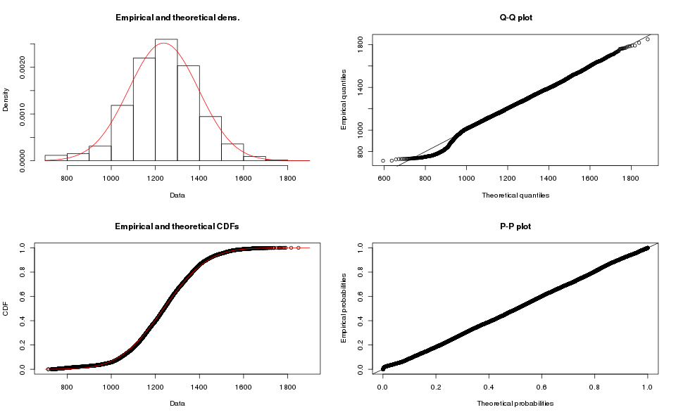
The Q-Q plot is a key step in the evaluation. You would want all (or most) of the dots to match the ideal line in the graph. The match is good except at the left side, where the samples kink out of the ideal line. Depending on the application you may accept this as a good enough fit. I am going to reject it because we see that the other set of samples (array-based) does not match the normal distribution either.
Is the Logistic Distribution a good fit for the Map-based data?
The Logistic distribution is also a close match for the map-based data.
m.logis.fit <- fitdist(m.data$microseconds, distr="logis")
plot(m.logis.fit)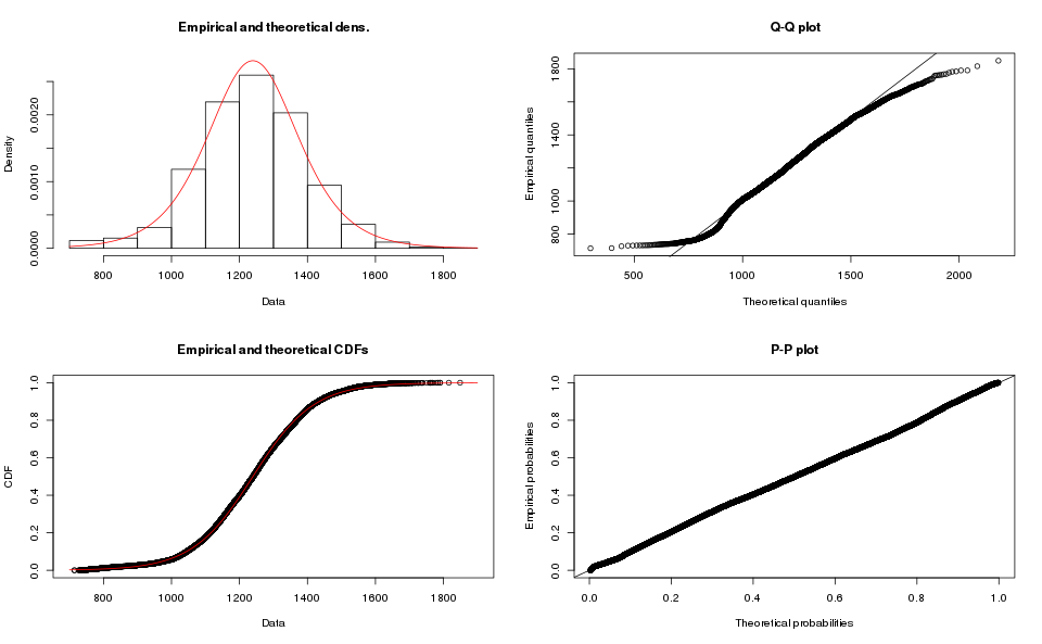
Clearly a poor match also.
Is the Gamma Distribution a Good Fit for the Array-based data?
The Gamma distribution family is not too far away from the data in the Cullen and Frey graph.
The operations in R are very similar (see the script for details), and the results for Array-based order book are:

While the results for Map-based order books are:
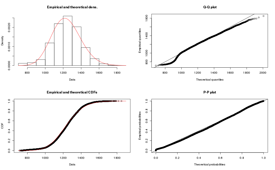
Clearly a poor fit for the map-based order book data, I do not like the tail on the Q-Q plot for the array-based order book.
What about the Beta Distribution?
The beta distribution would be a strange choice for this data, it only makes sense on the interval, and our data has a different domain. It also appears in ratios of probabilities, which would be really strange indeed. Purely to be thorough we scale down the data to the unit interval, and run the analysis:
m.data <- subset(data, book_type == 'map')
m.data$seconds <- m.data$microseconds / 1000000
a.data$seconds <- a.data$microseconds / 1000000
m.beta.fit <- fitdist(
m.data$seconds, distr="beta", start=beta.start(m.data$seconds))
plot(m.beta.fit)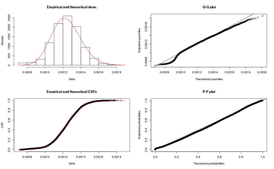
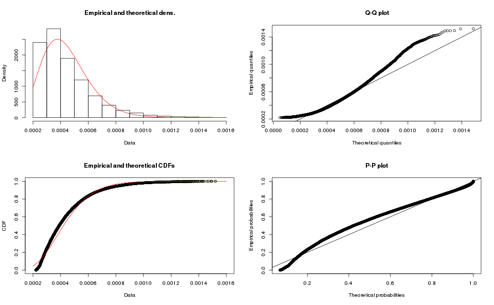
The graph clearly shows that this is a poor fit, and the KS-test confirms it:
m.beta.ks <- ks.test(x=m.data$seconds, y="beta", m.beta.fit$estimate)
m.beta.ks
One-sample Kolmogorov-Smirnov test
data: m.data$seconds
D = 965.77, p-value < 2.2e-16
alternative hypothesis: two-sidedThe results for the array-based samples is similar:
What about the Weibull Distribution?
The Weibull distribution seems a more plausible choice, it has been used to model delivery times, which might be an analogous problem.
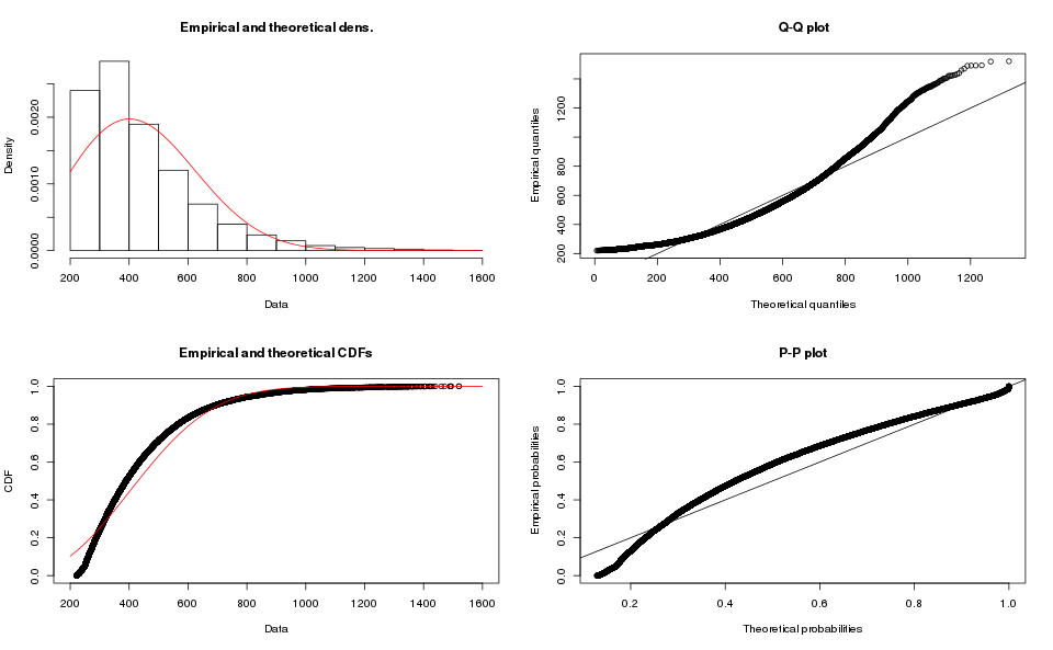
The operations in R are very similar (see the script for details), and the results for Array-based order book are:
While the results for Map-based order books are:
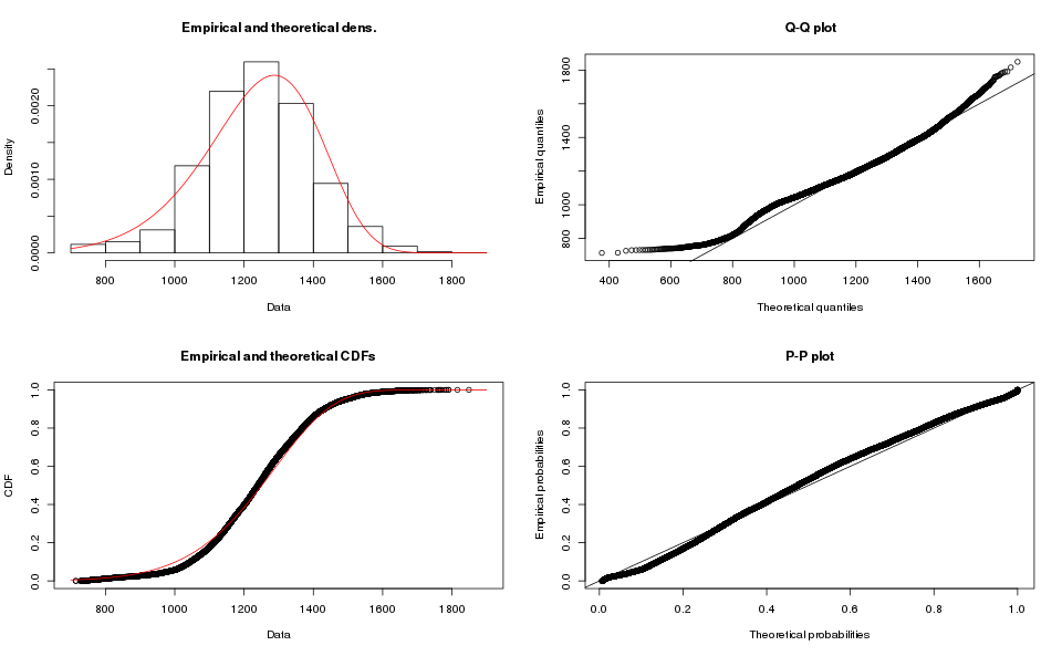
I do not think Weibull is a good fit either.
Instead of searching for more and more exotic distributions to test against I decided to go the distribution-free route.
Appendix Estimate Standard Deviation
Bootstrapping is the practice of estimating properties of an estimator (in our case the standard deviation) by resampling the data.
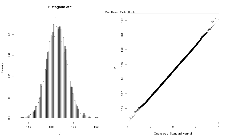
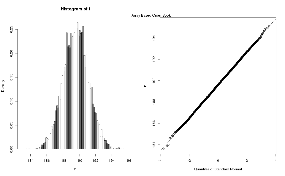
R provides a package for bootstrapping, we simply take advantage of it to produce the estimates. We reproduce here the bootstrap histograms, and Q-Q plots, they show the standard deviation estimator largely follow a normal distribution, and one can use the more economical methods to estimate the confidence interval (rounded down for min, rounded up for max):
| Book Type | Normal Method | Basic Method | Percentile Method |
|---|---|---|---|
| Map | (159.8, 160.3) | (156.8, 160.3) | (156.8, 160.3) |
| Array | (186.6, 192.7) | (186.6, 192.7) | (186.5, 192.7) |
Notice that the different methods largely agree with each other, which is a good sign that the estimates are good. We take the maximum of all the estimates, because we are using it for power analysis where the highest value is more conservative. After rounding up the maximum, we obtain as our estimate of the standard deviation for the purposes of power analysis.
Incidentally, this procedure confirmed that the number of samples used in the exploratory analysis was adequate. If we had taken an insufficient number of samples the estimated percentiles would have disagreed with each other.
Notes
The data for this post was generated using the driver script for the order book benchmark, with the e444f0f072c1e705d932f1c2173e8c39f7aeb663 version of JayBeams. The data thus generated was processed with a small R script to perform the statistical analysis and generate the graphs shown in this post. The R script as well as the data used here are available for download through the links.
Metadata about the tests, including platform details can be found in comments embedded with the data file. The highlights of that metadata is reproduced here:
- CPU: AMD A8-3870 CPU @ 3.0Ghz
- Memory: 16GiB DDR3 @ 1333 Mhz, in 4 DIMMs.
- Operating System: Linux (Fedora 23, 4.8.13-100.fc23.x86_64)
- C Library: glibc 2.22
- C++ Library: libstdc++-5.3.1-6.fc23.x86_64
- Compiler: gcc 5.3.1 20160406
- Compiler Options: -O3 -ffast-math -Wall -Wno-deprecated-declarations
Colophon
Unlike my prior posts, I used mostly raster images (PNG) for most of the graphs in this one. Unfortunately using SVG graphs broke my browser (Chrome), and it seemed to risky to include them. Until I figure out a way to safely offer SVG graphs, the reader can download them directly.