I recently became interested in using Kubernetes (aka k8s) to run
production services. One of the challenges I set for myself was to create a
relatively small Docker image for a C++ server of some sort. After some fiddling
with the development environment and tools I was able to create a 15MiB image
that contains both a server and a small client. This post describes how I got
this to work.
The Plan
My first idea was to create a minimal program, link it statically, and then copy
the program into the Docker image. In principle that should make the image
fairly small, a minimal Alpine Linux image is only 4MiB, if the
program is statically linked no other requirements are needed.
Unfortunately, most Linux distributions use glibc, which, for all practical purposes requires dynamic linking to support
“Name Service Switch” (NSS). Furthermore, glibc is licensed under the
GNU Lesser General Public License, and I do not want to
concern myself with the terms under which the binaries that statically link
glibc may or may not be redistributed. I am interested in writing code, not in
becoming a lawyer.
Fortunately Alpine Linux is based on the musl library, which
supports static linking without any of the glibc headaches.
To make the build easy to reproduce, we will first create a Docker image
containing all the development tools. I expect that this image will be rather
large, as the development tools, plus libraries, plus headers can take
significant space. The trick is to use Docker
multi-stage builds
to first compile the server using this large image, and then copy only the
server binary into a much smaller Docker image.
Setting up the Development Environment
Most of the libraries and tools I needed to compile my server were readily
available as Alpine Linux packages. So I just installed them using:
apk update && apk add build-base gcc g++
To get the static version of the C library you need to install one more package:
apk update && apk add libc-dev
I prefer to use Boost instead of writing my own libraries, so I
also installed the development version of Boost and the static version of these
libraries:
apk update && apk add boost-dev boost-static
I also prefer CMake as a meta-build system, and
Ninja as its backend:
apk update && apk add cmake ninja
Finally I will use vcpkg to install any dependencies that do not
have suitable Alpine Linux packages, so add some additional tools:
apk update && apk add curl git perl unzip tar
Compiling Additional dependencies
Some of the dependencies, such as gRPC, do not have readily available packages,
in this case I just use vcpkg to build them. First we need to download and
compile vcpkg itself:
git clone https://github.com/Microsoft/vcpkg.git
cd vcpkg
./bootstrap-vcpkg.sh --useSystemBinaries
Note that vcpkg can download the binaries it needs, such as CMake, or Perl, but
I decided to disable these downloads. Now we can compile the dependencies:
./vcpkg install --triplet x64-linux grpc
The triplet option is needed because vcpkg seems to default to a non-usable
triplet under Alpine Linux.
Compiling the gRPC server
With all the development tools in place I created a small project with a gRPC echo service.
This project is available from GitHub:
git clone https://github.com/coryan/docker-grpc-cpp.git
cd docker-grpc-cpp
I prefer CMake as by build tool for C++, in this case we need to provide a
number of special options:
I hope you found these instructions useful. I hope I will have time to describe
using an image such as the one created in this post to run a Kubernetes-based
service.
This is a long series of posts where I try to teach myself how to
run rigorous, reproducible microbenchmarks on Linux. You may
want to start from the first one
and learn with me as I go along.
I am certain to make mistakes, please write be back in
this bug when
I do.
In my previous post I chose the Mann-Whitney U
Test
to perform an statistical test of hypothesis comparing
array_based_order_book vs. map_based_order_book.
I also explored why neither the arithmetic mean, nor the median are
good measures of effect in this case.
I learned about the Hodges-Lehmann
Estimator
as a better measure of effect for performance improvement.
Finally I used some mock data to familiarize myself with these tools.
In this post I will solve the last remaining issue from my
Part 1 of this series.
Specifically [I12]: how can anybody reproduce the results
that I obtained.
The Challenge of Reproducibility
I have gone to some length to make the tests producible:
The code under test, and the code used to generate the results is
available from my github account.
The code includes full instructions to compile the system, and in
addition to the human readable documentation there are automated
scripts to compile the system.
I have also documented which specific version of the code was used
to generate each post, so a potential reader (maybe a future version
of myself), can fetch the specific version and rerun the tests.
Because compilation instructions can be stale, or incorrect, or hard
to follow,
I have made an effort to provide pre-packaged
docker images with
all the development tools and dependencies necessary to compile and
execute the benchmarks.
Despite these efforts I expect that it would be difficult, if not
impossible, to reproduce the results for a casual or even a persistent
reader: the exact hardware and software configuration that I used,
though documented, would be extremely hard to put together again.
Within months the packages used to compile and link the code will no
longer be current, and may even disappear from the repositories
where I fetched them from.
In addition, it would be quite a task to collect
the specific parts to reproduce a custom-built computer put together
several years ago.
I think containers may offer a practical way to package
the development environment, the binaries, and the analysis tools in a
form that allows us to reproduce the results easily.
I do not believe the reader would be able to reproduce the absolute
performance numbers, those depend closely on the physical hardware
used.
But one should be able to reproduce the main results, such as the
relative performance improvements, or the fact that we observed a
statistically significant improvement in performance.
I aim to explore these ideas in this post, though I cannot say that I
have fully solved the problems that arise when trying to use them.
Towards Reproducible Benchmarks
As part of its continuous integration builds JayBeams creates
runtime images with all the necessary code to run the benchmarks.
I have manually tagged the images that I used in this post, with the
post name, so they can be easily fetched.
Assuming you have a Linux workstation (or server), with docker
configured you should be able to execute the following commands to run
the benchmark:
The results will be generated in a local file named
bm_order_book_generate.1.results.csv.
You can verify I used the same version of the runtime image with the
following command:
The resulting report is included
later
in this post.
Running on Public Cloud Virtual Machines
Though the previous steps have addressed the problems with recreating
the software stack used to run the benchmarks I have not addressed the
problem of reproducing the hardware stack.
I thought I could solve this problem using public cloud, such as
Amazon Web Services,
or Google Cloud Platform.
Unfortunately I do not know (yet?) how to control the environment on a
public cloud virtual machine to avoid auto-correlation in the sample
data.
Below I will document the steps to run the benchmark on a virtual
machine,
but I should warn the reader upfront that the results are suspect.
The resulting report is included
later
in this post.
Create the Virtual Machine
I have chosen Google’s public cloud simply because I am more familiar
with it, I make no claims as to whether it is better or worse than the
alternatives.
# Set these environment variables based on your preferences# for Google Cloud Platform$ PROJECT=[your project name here]
$ ZONE=[your favorite zone here]
$ PROJECTID=$(gcloud projects --quiet list | grep$PROJECT | \
awk '{print $3}')# Create a virtual machine to run the benchmark$ VM=benchmark-runner
$ gcloud compute --project$PROJECT instances \
create $VM\--zone$ZONE--machine-type"n1-standard-2"--subnet"default"\--maintenance-policy"MIGRATE"\--scopes"https://www.googleapis.com/auth/cloud-platform"\--service-account\${PROJECTID}-compute@developer.gserviceaccount.com \--image"ubuntu-1604-xenial-v20170202"\--image-project"ubuntu-os-cloud"\--boot-disk-size"32"--boot-disk-type"pd-standard"\--boot-disk-device-name$VM
All that remains at this point is to describe how the images
themselves are created.
I automated the process to create images as part of the continuous
integration builds for JayBeams.
After each commit to the master
branch travis checks out the
code, uses an existing development environment to compile and test the
code, and then creates the runtime and analysis images.
If the runtime and analysis images differ from the existing images in
the github repository the new
images are automatically pushed to the github repository.
If necessary, a new development image is also created as part of the
continuous integration build.
This means that the development image might be one build behind,
as the latest runtime and analysis images may have been created with a
previous build image.
I have an outstanding
bug to fix this problem.
In practice this is not a major issue because the development
environment changes rarely.
An appendix to this post includes
step-by-step instructions on what the automated continuous integration
build does.
Tagging Images for Final Report
The only additional step is to tag the images used to create this
report, so they are not lost in the midst of time:
In this post I addressed the last remaining issue identified at the
beginning of this series.
I have made the tests as reproducible as I know how.
A reader can execute the tests in a public cloud server, or if they
prefer on their own Linux workstation, by downloading and executing
pre-compiled images.
It is impossible to predict for how long those images will remain
usable, but they certainly go a long way to make the tests and
analysis completely scripted.
Furthermore, the code to create the images themselves has been fully
automated.
Next Up
I will be taking a break from posting about benchmarks and statistics,
I want to go back to writing some code, more than talking about how to
measure code.
Notes
All the code for this post is available from the
78bdecd855aa9c25ce606cbe2f4ddaead35706f1
version of JayBeams, including the Dockerfiles used to create the
images.
The images themselves were automatically created using
travis.org, a service for continuous
integration.
The travis configuration file and helper script are also part of the
code for JayBeams.
Metadata about the tests, including platform details can be found in
comments embedded with the data files.
Appendix: Manual Image Creation
Normally the images are created by an automated build, but for
completeness we document the steps to create one of the runtime images
here.
We assume the system has been configured to run docker, and the
desired version of JayBeams has been checked out in the current
directory.
First we create a virtual machine, that guarantees that we do not have
hidden dependencies on previously installed tools or configurations:
Check Assumptions: Validate the Data is Independent
I inspect the data in case there are obvious problems with
independence of the samples.
Output as PNG files. While SVG files look better in a web page, large
SVG files tend to crash browsers.
I would like an analytical test to validate the samples are
indepedent,
a visual inspection of the data may help me detect obvious problems,
but I may miss more subtle issues.
For this part of the analysis it is easier to separate the data by
book type, so we create two timeseries for them:
I think any value higher than indicates that the samples are
not truly independent:
max.autocorrelation<-0.05if(max.acf.array>=max.autocorrelation|max.acf.map>=max.autocorrelation){warning("Some evidence of auto-correlation in ","the samples max.acf.array=",round(max.acf.array,4),", max.acf.map=",round(max.acf.map,4))}else{cat("PASSED: the samples do not exhibit high auto-correlation")}
## PASSED: the samples do not exhibit high auto-correlation
I am going to proceed, even though the data on virtual machines tends
to have high auto-correlation.
Power Analysis: Estimate Standard Deviation
Use bootstraping to estimate the standard deviation, we are going to
need a function to execute in the bootstrapping procedure:
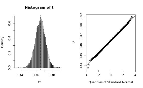
We need to verify that the estimated statistic roughly follows a
normal distribution, otherwise the bootstrapping procedure would
require a lot more memory than we have available:
The Q-Q plots look reasonable, so we can estimate the standard
deviation using a simple procedure:
Power Analysis: Determine Required Number of Samples
We need to determine if the sample size was large enough given the
estimated standard deviation, the expected effect size, and the
statistical test we are planning to use.
The is the minimum effect size that we could be interested in is based
on saving at least one cycle per operation in the classes we are
measuring.
The test executes 20,000 iterations:
test.iterations<-20000
and we assume that the clock cycle is approximately 3Ghz:
clock.ghz<-3
We can use this to compute the minimum interesting effect:
That is, any result smaller than 6.6667 microseconds would not
be interesting and should be rejected.
We need a few more details to compute the minimum number of samples,
first, the desired significance of any results, which we set to:
desired.significance<-0.01
Then, the desired statistical power of the test, which we set to:
desired.power<-0.95
We are going to use a non-parametric test, which has a 15% overhead
above the t-test:
nonparametric.extra.cost<-1.15
In any case, we will require at least 5000 iterations, because it is
relatively fast to run that many:
min.samples<-5000
If we do not have enough power to detect 10 times the minimum effect
we abort the analysis, while if we do not have enough samples to
detect the minimum effect we simply generate warnings:
##
##      Two-sample t test power calculation
##
##               n = 312.8
##           delta = 66.67
##              sd = 197
##       sig.level = 0.01
##           power = 0.95
##     alternative = two.sided
##
## NOTE: n is number in *each* group
We are going to round the number of iterations to the next higher
multiple of 1000, because it is easier to type, say, and reason about
nice round numbers:
That is, we need 5000 samples to detect an effect of
66.67 microseconds at the desired significance
and power levels.
if(required.nsamples>length(data.array.ts)){stop("Not enough samples in 'array' data to"," detect expected effect (",10*min.delta,") should be >=",required.nsamples," actual=",length(array.map.ts))}if(required.nsamples>length(data.map.ts)){stop("Not enough samples in 'map' data to"," detect expected effect (",10*min.delta,") should be >=",required.nsamples," actual=",length(map.map.ts))}
##
##      Two-sample t test power calculation
##
##               n = 31112
##           delta = 6.667
##              sd = 197
##       sig.level = 0.01
##           power = 0.95
##     alternative = two.sided
##
## NOTE: n is number in *each* group
That is, we need at least 36000
samples to detect the minimum interesting effect of 6.6667
microseconds.
Notice that our tests have 35000 samples.
if(desired.nsamples>length(data.array.ts)|desired.nsamples>length(data.map.ts)){warning("Not enough samples in the data to"," detect the minimum interating effect (",round(min.delta,2),") should be >= ",desired.nsamples," map-actual=",length(data.map.ts)," array-actual=",length(data.array.ts))}else{cat("PASSED: The samples have the minimum required power")}
## Warning: Not enough samples in the data to detect the
## minimum interating effect (6.67) should be >= 36000 map-
## actual=35000 array-actual=35000
The estimated effect is -771.5501 microseconds, if this
number is too small we need to stop the analysis:
if(abs(estimated.delta)<min.delta){stop("The estimated effect is too small to"," draw any conclusions."," Estimated effect=",estimated.delta," minimum effect=",min.delta)}else{cat("PASSED: the estimated effect (",round(estimated.delta,2),") is large enough.")}
## PASSED: the estimated effect ( -771.5 ) is large enough.
Finally, the p-value determines if we can reject the null hypothesis
at the desired significance.
In our case, failure to reject means that we do not have enough
evidence to assert that the array_based_order_book is faster or
slower than map_based_order_book.
If we do reject the null hypothesis then we can use the
Hodges-Lehmann estimator
to size the difference in performance,
aka the effect of our code changes.
if(data.mw$p.value>=desired.significance){cat("The test p-value (",round(data.mw$p.value,4),") is larger than the desired\n","significance level of alpha=",round(desired.significance,4),"\n",sep="")cat("Therefore we CANNOT REJECT the null hypothesis"," that both the 'array'\n","and 'map' based order books have the same"," performance.\n",sep="")}else{interval<-paste0(round(data.mw$conf.int,2),collapse=',')cat("The test p-value (",round(data.mw$p.value,4),") is smaller than the desired\n","significance level of alpha=",round(desired.significance,4),"\n",sep="")cat("Therefore we REJECT the null hypothesis that"," both the\n"," 'array' and 'map' based order books have\n","the same performance.\n",sep="")cat("The effect is quantified using the Hodges-Lehmann\n","estimator, which is compatible with the\n","Mann-Whitney U test, the estimator value\n","is ",round(data.mw$estimate,2)," microseconds with a 95% confidence\n","interval of [",interval,"]\n",sep="")}
## The test p-value (0) is smaller than the desired
## significance level of alpha=0.01
## Therefore we REJECT the null hypothesis that both the
##  'array' and 'map' based order books have
## the same performance.
## The effect is quantified using the Hodges-Lehmann
## estimator, which is compatible with the
## Mann-Whitney U test, the estimator value
## is -771.5 microseconds with a 95% confidence
## interval of [-773.77,-769.32]
Mini-Colophon
This report was generated using knitr
the details of the R environment are:
library(devtools)devtools::session_info()
## Session info -----------------------------------------------
##  setting  value
##  version  R version 3.2.3 (2015-12-10)
##  system   x86_64, linux-gnu
##  ui       X11
##  language (EN)
##  collate  C
##  tz       Zulu
##  date     2017-02-20
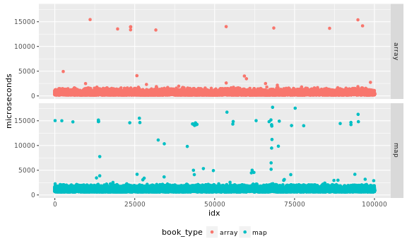
Check Assumptions: Validate the Data is Independent
I inspect the data in case there are obvious problems with
independence of the samples.
Output as PNG files. While SVG files look better in a web page, large
SVG files tend to crash browsers.
I would like an analytical test to validate the samples are
indepedent,
a visual inspection of the data may help me detect obvious problems,
but I may miss more subtle issues.
For this part of the analysis it is easier to separate the data by
book type, so we create two timeseries for them:
I think any value higher than indicates that the samples are
not truly independent:
max.autocorrelation<-0.05if(max.acf.array>=max.autocorrelation|max.acf.map>=max.autocorrelation){warning("Some evidence of auto-correlation in ","the samples max.acf.array=",round(max.acf.array,4),", max.acf.map=",round(max.acf.map,4))}else{cat("PASSED: the samples do not exhibit high auto-correlation")}
## Warning: Some evidence of auto-correlation in the samples
## max.acf.array=0.0964, max.acf.map=0.256
I am going to proceed, even though the data on virtual machines tends
to have high auto-correlation.
Power Analysis: Estimate Standard Deviation
Use bootstraping to estimate the standard deviation, we are going to
need a function to execute in the bootstrapping procedure:
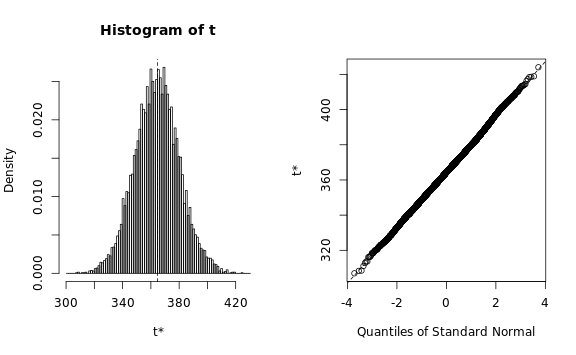
We need to verify that the estimated statistic roughly follows a
normal distribution, otherwise the bootstrapping procedure would
require a lot more memory than we have available:
The Q-Q plots look reasonable, so we can estimate the standard
deviation using a simple procedure:
Power Analysis: Determine Required Number of Samples
We need to determine if the sample size was large enough given the
estimated standard deviation, the expected effect size, and the
statistical test we are planning to use.
The is the minimum effect size that we could be interested in is based
on saving at least one cycle per operation in the classes we are
measuring.
The test executes 20,000 iterations:
test.iterations<-20000
and we assume that the clock cycle is approximately 3Ghz:
clock.ghz<-3
We can use this to compute the minimum interesting effect:
That is, any result smaller than 6.6667 microseconds would not
be interesting and should be rejected.
We need a few more details to compute the minimum number of samples,
first, the desired significance of any results, which we set to:
desired.significance<-0.01
Then, the desired statistical power of the test, which we set to:
desired.power<-0.95
We are going to use a non-parametric test, which has a 15% overhead
above the t-test:
nonparametric.extra.cost<-1.15
In any case, we will require at least 5000 iterations, because it is
relatively fast to run that many:
min.samples<-5000
If we do not have enough power to detect 10 times the minimum effect
we abort the analysis, while if we do not have enough samples to
detect the minimum effect we simply generate warnings:
##
##      Two-sample t test power calculation
##
##               n = 1259
##           delta = 66.67
##              sd = 396
##       sig.level = 0.01
##           power = 0.95
##     alternative = two.sided
##
## NOTE: n is number in *each* group
We are going to round the number of iterations to the next higher
multiple of 1000, because it is easier to type, say, and reason about
nice round numbers:
That is, we need 5000 samples to detect an effect of
66.67 microseconds at the desired significance
and power levels.
if(required.nsamples>length(data.array.ts)){stop("Not enough samples in 'array' data to"," detect expected effect (",10*min.delta,") should be >=",required.nsamples," actual=",length(array.map.ts))}if(required.nsamples>length(data.map.ts)){stop("Not enough samples in 'map' data to"," detect expected effect (",10*min.delta,") should be >=",required.nsamples," actual=",length(map.map.ts))}
##
##      Two-sample t test power calculation
##
##               n = 125711
##           delta = 6.667
##              sd = 396
##       sig.level = 0.01
##           power = 0.95
##     alternative = two.sided
##
## NOTE: n is number in *each* group
That is, we need at least 145000
samples to detect the minimum interesting effect of 6.6667
microseconds.
Notice that our tests have 100000 samples.
if(desired.nsamples>length(data.array.ts)|desired.nsamples>length(data.map.ts)){warning("Not enough samples in the data to"," detect the minimum interating effect (",round(min.delta,2),") should be >= ",desired.nsamples," map-actual=",length(data.map.ts)," array-actual=",length(data.array.ts))}else{cat("PASSED: The samples have the minimum required power")}
## Warning: Not enough samples in the data to detect the
## minimum interating effect (6.67) should be >= 145000 map-
## actual=100000 array-actual=100000
The estimated effect is -600.7931 microseconds, if this
number is too small we need to stop the analysis:
if(abs(estimated.delta)<min.delta){stop("The estimated effect is too small to"," draw any conclusions."," Estimated effect=",estimated.delta," minimum effect=",min.delta)}else{cat("PASSED: the estimated effect (",round(estimated.delta,2),") is large enough.")}
## PASSED: the estimated effect ( -600.8 ) is large enough.
Finally, the p-value determines if we can reject the null hypothesis
at the desired significance.
In our case, failure to reject means that we do not have enough
evidence to assert that the array_based_order_book is faster or
slower than map_based_order_book.
If we do reject the null hypothesis then we can use the
Hodges-Lehmann estimator
to size the difference in performance,
aka the effect of our code changes.
if(data.mw$p.value>=desired.significance){cat("The test p-value (",round(data.mw$p.value,4),") is larger than the desired\n","significance level of alpha=",round(desired.significance,4),"\n",sep="")cat("Therefore we CANNOT REJECT the null hypothesis"," that both the 'array'\n","and 'map' based order books have the same"," performance.\n",sep="")}else{interval<-paste0(round(data.mw$conf.int,2),collapse=',')cat("The test p-value (",round(data.mw$p.value,4),") is smaller than the desired\n","significance level of alpha=",round(desired.significance,4),"\n",sep="")cat("Therefore we REJECT the null hypothesis that"," both the\n"," 'array' and 'map' based order books have\n","the same performance.\n",sep="")cat("The effect is quantified using the Hodges-Lehmann\n","estimator, which is compatible with the\n","Mann-Whitney U test, the estimator value\n","is ",round(data.mw$estimate,2)," microseconds with a 95% confidence\n","interval of [",interval,"]\n",sep="")}
## The test p-value (0) is smaller than the desired
## significance level of alpha=0.01
## Therefore we REJECT the null hypothesis that both the
##  'array' and 'map' based order books have
## the same performance.
## The effect is quantified using the Hodges-Lehmann
## estimator, which is compatible with the
## Mann-Whitney U test, the estimator value
## is -600.8 microseconds with a 95% confidence
## interval of [-602.48,-599.11]
Mini-Colophon
This report was generated using knitr
the details of the R environment are:
library(devtools)devtools::session_info()
## Session info -----------------------------------------------
##  setting  value
##  version  R version 3.2.3 (2015-12-10)
##  system   x86_64, linux-gnu
##  ui       X11
##  language (EN)
##  collate  C
##  tz       Zulu
##  date     2017-02-20
This is a long series of posts where I try to teach myself how to
run rigorous, reproducible microbenchmarks on Linux. You may
want to start from the first one
and learn with me as I go along.
I am certain to make mistakes, please write be back in
this bug when
I do.
In my previous post I convinced myself that
the data we are dealing with does not fit the most common
distributions such as normal, exponential or lognormal,
and therefore I decided to use nonparametric statistics to analyze the
data.
I also used power analysis to determine the number of samples
necessary to have high confidence in the results.
In this post I will choose the statistical test of hypothesis,
and verify that the assumptions for the test hold.
I will also familiarize myself with the test by using some mock data.
This will address two of the issues raised in
Part 1 of this series.
Specifically [I10]: the lack of statistical significance
in the results, in other words, whether they can be explained by luck
alone or not, and [I11]: justifying how I select the
statistic to measure the effect.
Modeling the Problem
I need to turn the original problem into the language of statistics,
if the reader recalls, I want to compare the performance of two
classes in JayBeams:
array_based_order_book against
map_based_order_book,
and determine if they are really different or the results can be
explained by luck.
I am going to model the performance results as random variables,
I will use for the performance results (the running time of the
benchmark) of array_based_order_book and for
map_based_order_book.
If all we wanted to compare was the mean of these random variables
I could use
Student’s t-test.
While the underlying distributions are not normal, the test only
requires [1]
that the statistic you compare follows the normal distribution.
The (difference of)means most likely distributes normal for large samples,
as the CLT
applies in a wide range of circumstances.
But I have convinced myself, and hopefully the reader, that
the mean is not a great statistic for this type of data.
It is not a robust statistic, and outliers should be common because of
the long tail in the data.
I would prefer a more robust test.
The Mann-Whitney U
Test
is often recommended when the underlying distributions are not normal.
It can be used to test the hypothesis that
which is exactly what I am looking for.
I want to assert that it is more likely that array_based_order_book
will run faster than map_based_order_book.
I do not need to assert that it is always faster, just that it is a
good bet that it is.
The Mann-Whitney U test also requires me to make a relatively weak set
of assumptions, which I will check next.
Assumption: The responses are ordinal This is trivial, the
responses are real numbers that can be readily sorted.
Assumption: Null Hypothesis is of the right form I define the null
hypothesis to match the requirements of the test:
Intuitively this definition is saying that the code changes
had no effect, that both versions have the same probability of being
faster than the other.
Assumption: Alternative Hypothesis is of the right form I define
the alternative hypothesis to match the assumptions of the
test:
Notice that this is weaker than what I would like to assert:
As we will see in the
Appendix
that alternative hypothesis requires additional assumptions that I
cannot make, specifically that the two distributions only differ by
some location parameter.
Assumption: Random Samples from Populations The test assumes the
samples are random and extracted from a single population.
It would be really bad, for example, if I grabbed half my samples from
one population and half from another,
that would break the “identically distributed” assumption that almost
any statistical procedure requires.
It would also be a “Bad Thing”[tm] if my samples were biased in any
way.
I think the issue of sampling from a single population is trivial, by
definition we are extracting samples from one population.
I have already discussed the problems in biasing that my approach has.
while not perfect, I believe it to be good enough for the time being,
and will proceed under the assumption that no biases exist.
Assumption: All the observations are independent of each other I
left the more difficult one for last.
This is a non-trivial assumption in my case because one can reasonably
argue that result of one experiment may affect the results of the next
one.
Running the benchmark populates the instruction and data cache,
affects the state of the memory arena,
and may change the
P-state
of the CPU.
Furthermore, the samples are generated using a PRNG, if the generator
was chosen poorly the samples may be auto-correlated.
So I need to perform at least a basic test for independence of the
samples.
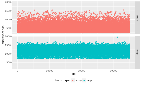
Checking Independence
To check independence I first plot the raw results:
Uh oh, those drops and peaks are not single points, there seems to be
periods of time when the test runs faster or slower. That does not
bode well for an independence test.
I will use a correlogram
to examine if the data shows any auto-correlation:
That is a lot of auto-correlation. What is wrong?
After a long chase suspecting my random number generators I finally
identified the
bug
I had accidentally disabled the CPU frequency scaling settings in the
benchmark driver.
The data is auto-correlated because sometimes the load
generated by the benchmark changes the P-state of the processor, and
that affects several future results.
A quick
fix
to set the P-state to a fixed value, and the results look much better:
Other than the trivial autocorrelation at lag 0, the maximum
autocorrelation for map and array is , that seems acceptably
low to me.
Measuring the Effect
I have not yet declared how we are going to measure the effect.
The standard statistic to use in conjunction with Mann-Whitney U test is the
Hodges-Lehmann
Estimator.
Its definition is relatively simple: take all the pairs formed by
taking one sample from and one sample from , compute the
differences of each pair, then compute the median of those
differences, that is the value of the estimator.
Intuitively, if is the value of the Hodges-Lehmann
estimator then we can say that at least 50% of the time
and – if is negative – then at least 50% of the time the
array_based_order_book is faster than map_based_order_book.
I have to be careful, because I cannot make assertions about all of
the time. It is possible that the p51 of those differences of pairs
is a large positive number, and we will see in the
Appendix that
such results are quite possible.
Applying the Test
Applying the statistical test is a bit of an anti-climax.
But let’s recall what we are about to do:
The results are only interesting if the effect, as measured by
the Hodges-Lehmann Estimator is larger than the minimum desired
effect, which I set to in a previous post.
The test needs at least 35,000 iterations to be sufficiently
powered () to detect that effect at a significance level
of , as long as the estimated standard
deviation is less than .
We are going to use the Mann-Whitney U test to test the null
hypothesis that both distributions are identical.
The estimated effect is, therefore, at least .
We verify that the estimated standard deviations are small enough to
keep the test sufficiently powered:
BOOTSTRAP CONFIDENCE INTERVAL CALCULATIONS
Based on 10000 bootstrap replicates

CALL :
boot.ci(boot.out = data.map.sd.boot, type = c("perc", "norm", "basic"))

Intervals :
Level      Normal              Basic              Percentile
95%   (154.6, 157.1 )   (154.6, 157.1 )   (154.6, 157.1 )
Calculations and Intervals on Original Scale
So all assumptions are met to run the hypothesis test.
R calls this test wilcox.test() because there is no general
agreement on the literature about whether “Mann-Whitney U test” or
“Wilcoxon Rank Sum” is the correct name, regardless, running the test
is easy:
	Wilcoxon rank sum test with continuity correction

data:  microseconds by book_type
W = 7902700, p-value < 2.2e-16
alternative hypothesis: true location shift is not equal to 0
Therefore we can reject the null hypothesis that
at the confidence level.
Summary
I have addressed one of the remaining issues from the first post in
the series:
[I10] I have provided a comparison of the performance of
array_based_order_book against map_based_order_book, based on the
Mann-Whitney U test, and shown that these results are very likely not
explained by luck alone.
I verified that the problem matches the necessary assumptions of the
Mann-Whitney U test, and found a bug in my test framework in the
process.
[I11] I used the Hodges-Lehmann estimator to measure the
effect, mostly because it is the recommended estimator for the
Mann-Whitney U test. In an
Appendix
I show how this estimator is better than the difference of means and
the difference of medians for this type of data.
Next Up
In the next post I would like to show how to completely automate
the executions of such benchmarks, and make it possible to any reader
to run the tests themselves.
Appendix: Familiarizing with the Mann-Whitney Test
I find it useful to test new statistical tools with fake data to
familiarize myself with them.
I also think it is useful to gain some understand of what the results
should be in ideal conditions, so we can interpret the results of live
conditions better.
The trivial test
I asked R to generate some random samples for me, fitting the
Lognormal
distribution.
I picked Lognormal because, if you squint really hard, it looks
vaguely like latency data:
I always try to see what a statistical test says when I feed it
identical data on both sides. One should expect the test to fail to
reject the null hypothesis in this case, because the null hypothesis
is that both sets are the same.
If you find the language of statistical testing somewhat convoluted
(e.g. “fail to reject” instead of simple “accept”), you are not alone,
I think that is the sad cost of rigor.
	Wilcoxon rank sum test with continuity correction

data:  lnorm.s1 and lnorm.s1
W = 1.25e+09, p-value = 1
alternative hypothesis: true location shift is not equal to 0
95 percent confidence interval:
 -0.3711732  0.3711731
sample estimates:
difference in location
         -6.243272e-08
That seems like a reasonable answer, the p-value is about as high as
it can get, and the estimate of the location parameter difference is
close to 0.
Two Samples from the same Distribution
I next try with a second sample from the same distribution, the test
should fail to reject the null again, and the estimate should be close
to 0:
Wilcoxon rank sum test with continuity correction

data:  lnorm.s1 and lnorm.s2
W = 1252400000, p-value = 0.5975
alternative hypothesis: true location shift is not equal to 0
95 percent confidence interval:
 -0.2713750  0.4712574
sample estimates:
difference in location
            0.09992599
That seems like a good answer too. Conventionally the one fails to
reject the null if the p-value is above 0.01 or 0.05.
The output of the test is telling us that under the null hypothesis
one would obtain this result (or something more extreme) of
the time.
That seems pretty good odds to reject the null indeed.
Notice that the estimate for the location parameter difference is not
zero (which we know to be the true value), but the confidence interval
does include 0.
Statistical Power Revisited
Okay, so this test seems to give sensible answers when we give it data
from identical distributions.
What I want to do is try it with different distributions, let’s start
with something super simple: two distributions that are slightly
shifted from each other:
	Wilcoxon rank sum test with continuity correction

data:  lnorm.s3 and lnorm.s4
W = 1249300000, p-value = 0.8718
alternative hypothesis: true location shift is not equal to 0
95 percent confidence interval:
 -0.4038061  0.3425407
sample estimates:
difference in location
           -0.03069523
Hmmm… Ideally we would have rejected the null in this case,
but we cannot (p-value is higher than my typical 0.01 significance
level).
What is
going on? And why does the 95% confidence interval for the estimate
includes 0? We know the difference is 0.1.
I “forgot” to do power analysis again. This test is not sufficiently
powered:
     Two-sample t test power calculation

              n = 1486639
          delta = 0.1
             sd = 30.77399
      sig.level = 0.05
          power = 0.8
    alternative = two.sided

NOTE: n is number in *each* group
Ugh, we would need about 1.5 million samples to reliably detect an
effect the size of our small 0.1 shift. How much can we detect with
about 50,000 samples?
	Wilcoxon rank sum test with continuity correction

data:  lnorm.s5 and lnorm.s6
W = 1220100000, p-value = 5.454e-11
alternative hypothesis: true location shift is not equal to 0
95 percent confidence interval:
 -1.6227139 -0.8759441
sample estimates:
difference in location
             -1.249286
It is working again! Now I can reject the null hypothesis at the
0.01 level (p-value is much smaller than that).
The effect estimate is -1.24, and we know the test is powered enough
to detect that.
We also know (now) that the test basically estimates the location
parameter of the x series against the second series.
Better Accuracy for the Test
The parameter estimate is not very accurate though, the true parameter
is -1.0, we got -1.24. Yes, the true value falls in the 95%
confidence interval, but how can we make that interval smaller?
We can either increase the number of samples or
the effect, let’s go with the effect:
	Wilcoxon rank sum test with continuity correction

data:  lnorm.s7 and lnorm.s8
W = 1136100000, p-value < 2.2e-16
alternative hypothesis: true location shift is not equal to 0
95 percent confidence interval:
 -5.110127 -4.367495
sample estimates:
difference in location
             -4.738913
I think the lesson here is that for better estimates of the parameter
you need to have a sample count much higher than the minimum required
to detect that effect size.
Testing with Mixed Distributions
So far we have been using a very simple Lognormal distribution, I
know the test data is more difficult than this, I rejected a number of
standard distributions in the previous post.
First we create a function to generate random samples from a mix of
distributions:
rmixed<-function(n,shape=0.2,scale=2000){g1<-rlnorm(0.7*n,sdlog=shape)g2<-1.0+rlnorm(0.2*n,sdlog=shape)g3<-3.0+rlnorm(0.1*n,sdlog=shape)v<-scale*append(append(g1,g2),g3)## Generate a random permutation, otherwise g1, g2, and g3 are in## order in the vectorreturn(sample(v))}
And then we select a few samples using that distribution:
That is more interesting, admittedly not as difficult as the
distribution from our benchmarks, but at least not trivial.
I would like to know how many samples to take to measure an effect of
, which requires computing the standard deviation of the mixed
distribution.
I use bootstrapping to obtain an estimate:
With the estimated standard deviation out of the way, I can compute
the required number of samples to achieve a certain power and
significance level. I am picking 0.95 and 0.01, respectively:
	Wilcoxon rank sum test with continuity correction

data:  mixed.s1 and mixed.s2
W = 1728600000, p-value < 2.2e-16
alternative hypothesis: true location shift is not equal to 0
95 percent confidence interval:
 -60.18539 -43.18903
sample estimates:
difference in location
             -51.68857
That provides the answer I was expecting, the estimate for the
difference in the location parameter ()
is fairly close to the true value of .
More than the Location Parameter
So far I have been using simple translations of the same distribution,
the Mann-Whitnet U test is most powerful in that case.
I want to demonstrate the limitations of the test when the two random
variables differ by more than just a location parameter.
	Wilcoxon rank sum test with continuity correction

data:  value by sample
W = 998860000, p-value < 2.2e-16
alternative hypothesis: true location shift is not equal to 0
95 percent confidence interval:
 -581.5053 -567.7730
sample estimates:
difference in location
             -574.6352
R dutifully produces an estimate of the difference in location,
because I asked for it, but not because it has any reasonable
interpretation beyond “this is the median of the differences”.
Looking at the cumulative histogram we can see that sometimes s1 is
“faster” than s2, but the opposite is also true:
I also found it useful to plot the density of the differences:
This shows that while the Hodges-Lehmann estimator is negative, and
significant, that is not the end of the story, many samples are
higher.
I should be careful in how I interpret the results of the Mann-Whitney
U test when the distributions differ by more than just a location
parameter.
Appendix: Learning about the Hodges-Lehmann Estimator
Just like I did for the Mann-Whitney U test, I am going to use
synthetic data to gain some intuition about how it works.
I will try to test some of the better known estimators and see how
they break down, and compare how Hodges-Lehmann works in those cases.
Comparing Hodges-Lehmann vs. Difference of Means
I will start with a mixed distribution that includes mostly data
following a Lognormal distribution, but also includes some outliers.
This is what I expect to find in benchmarks that have not controlled
their execution environment very well:
I think this is a good time to point out that the Hodges-Lehmann
estimator of two samples is not the same as the difference of the
Hodges-Lehmann estimator of each sample:
print(HodgesLehmann(o2)-HodgesLehmann(o1))
[1] -2.908595
Basically Hodges-Lehmann for one sample is the median of averages
between pairs from the sample. For two samples it is the median of
the differences.
Comparing Hodges-Lehmann vs. the Difference of Medians
As I suspected, the difference of means is not a great estimator of
effect, it is not robust against outliers. What about the difference
of the medians? Seems to work fine in the previous case.
The example that gave me the most insight into why the median is not
as good as I thought is this:
The median of both is very similar, in fact o3 seems to have a worse
median:
print(median(o3)-median(o4))
[1] 11.32098
But clearly o3 has better performance.
Unfortunately the median cannot detect that, the same thing that makes
it robust against outliers makes it insensitive to changes in the top
50% of the data.
One might be tempted to use the mean instead, but we already know that
the problems are there.
The Hodges-Lehmann estimator readily detects the improvement:
print(HodgesLehmann(o3,o4))
[1] -1020.568
I cannot claim that the Hodges-Lehmann estimator will work well in all
cases.
But I think it offers a nice combination of being robust against
outliers, while sensitive to improvements in only part of the
population.
The
definition
is a bit hard to get used to,
but it matches what I think it is interesting in a benchmark:
if I run with approach A vs. approach B, will be A faster than B most
of the time? And if so, by how much?
Notes
The data for this post was generated using the
driver script
for the order book benchmark,
with the
e444f0f072c1e705d932f1c2173e8c39f7aeb663
version of JayBeams.
The data thus generated was processed with a small R
script to perform the
statistical analysis and generate the graphs shown in this post.
The R script as well as the
data used here are available for
download.
Metadata about the tests, including platform details can be found in
comments embedded with the data file.
The highlights of that metadata is reproduced here:
CPU: AMD A8-3870 CPU @ 3.0Ghz
Memory: 16GiB DDR3 @ 1333 Mhz, in 4 DIMMs.
Operating System: Linux (Fedora 23, 4.8.13-100.fc23.x86_64)
The data and graphs in the
Appendix
is randomly generated, the reader will not get the same results I did
when executing the script to generate those graphs.
This is a long series of posts where I try to teach myself how to
run rigorous, reproducible microbenchmarks on Linux. You may
want to start from the first one
and learn with me as I go along.
I am certain to make mistakes, please write be back in
this bug when
I do.
In my previous post I framed the
performance evaluation of array_based_order_book_side<> vs.
map_based_order_book_side<> as a statistical hypothesis testing problem.
I defined the minimum effect that would of interest, operationalized
the notion of “performance”, and defined the population of interest.
I think the process of formally framing the performance evaluation can
be applied to any CPU-bound algorithm or data structure,
and it can yield interesting observations.
For example, as I wrote down the population and problem statement it
became apparent that I had designed the benchmark improperly.
It was not sampling a large enough population of inputs,
or at least it was cumbersome to use it to generate a large sample
like this.
In this post I review an improved version of the benchmark, and do
some exploratory data analysis to prepare for our formal data capture.
Updates
I found a bug in the driver script for the benchmark, and updated
the results after fixing the bug. None of the main conclusions
changed, the tests simply got more consistent, with lower standard
deviation.
The New Benchmark
I implemented three changes to the benchmark, first I modified the
program to generate a new input sequence on each iteration.
Then I modified the program to randomly select which side of the book
the iteration was going to test.
Finally, I modified the benchmark to pick the first order at random as
opposed to use convenient but hard-coded values.
To modify the input data on each iteration I just added
iteration_setup() and iteration_teardown() member functions to the
benchmarking fixture.
With a little extra programming
fun
I modified the
microbenchmark framework to only call those functions if they are
present.
Modifying the benchmark created a bit of programming fun.
The code uses static polymorphism to represent buy vs. sell sides of
the book, and I wanted to randomly select one vs. the other.
With a bit of
type erasure the task is
completed.
Biases in the Data Collection
I paid more attention to the
seeding
of my PRNG, because I do not want to introduce biases in the
sampling.
While this is a obvious improvement this got me thinking about any
other biases in the sampling.
I think there might be problems with bias, but that needs some
detailed explanation of the procedure.
I think the
code
speaks better than I could, so I refer the reader to it.
The TL;DR; version for those who would rather not read code:
I generate a sequence of operations incrementally.
To create a new operation pick a price level based on the distribution
of event depths I measured for real data, just make sure the operation
is a legal change to the book.
Keep track of the book implied by all these operations.
At the end verify the distribution passes the criteria I set earlier
in this series (p99.9 within a given range), regenerate the series
from scratch if it fails the test.
Characterizing if this is a bias sampler or not would be an extremely
difficult problem to tackle,
for example, the probability of seeing any particular sequence of
operations in the wild is unknown, beyond the characterization of the
event depth distribution I found earlier.
Nor do I have a good characterization of the quantities.
I think the major problem is that the sequences generated by the
code
tend to meet the event depth distribution at every length,
while the sequences in the wild may converge only slowly to the
observed distribution of event depths.
This is arguably a severe pitfall in the analysis.
Effectively it limits the results to “for the population of inputs
that can be reached by the code to generate synthetic inputs”.
Nevertheless, that set of inputs is rather large, and I think a much
better approximation to what one would find “in the wild” than those
generated by any other source I know of.
I will proceed and caveat the results accordingly.
Exploring the Data
This is standard fare in statistics, before you do any kind of formal
analysis check what the data looks like, do some exploratory analysis.
That will guide your selection of model, the type of statistical tests
you will use, how much data to collect, etc.
The important thing is to discard that data at the end,
otherwise you might discover interesting things that are not actually
there.
I used the microbenchmark to take samples for each of the
implementations (map_based_order_book and array_based_order_book).
The number of samples is somewhat arbitrary, but we do confirm in an
appendix that is is high enough.
The first thing I want to look at is the distribution of the data,
just to get a sense of how it is shaped:
The first observation is that the data for map-based order books does
not look like any of the distributions I am familiar with.
The array-based order book may be
log normal
, or maybe Weibull.
Clearly none of them is a
normal distribution,
too much skew.
Nor do they look
exponential,
they don’t peak at 0.
This is getting tedious though, fortunately there is a nice tool to
check multiple distributions at the same time:
What these graphs are showing is how closely the sample
skewness
and kurtosis
would match the skewness and kurtosis of several commonly used
distributions.
For example, it seems the map-based order book closely matches the
skweness and kurtosis for a normal or
logistic
distribution.
Likewise, the array-based order book might match the
gamma distribution
distribution family – represented by the dashed line –
or it might be fitted to the beta distribution.
From the graphs it is not obvious if the
Weibull
distribution would be a good fit.
I made a more detailed analysis in the
Goodness of Fit
appendix,
suffice is to say that none of the common distributions are a good fit.
All this means is that we need to dig deeper into the statistics
toolbox, and use
nonparametric
(or if you prefer distribution free) methods.
The disadvantage of nonparametric methods is that they often require
more computation,
but computation is nearly free these days.
Their advantage is that one can operate with minimal assumptions about
the underlying distribution.
Yay! I guess?
Power Analysis
The first question to answer before we start collecting data is how
much data we want to collect?
If our data followed the normal distribution this would be an easy
exercise in statistical power analysis: you are going to use the
Student’s t-test,
and there are good functions in any statistical package to determine
how many samples you need to achieve a certain statistical power.
The Student’s t-test requires that the statistic being compared follows
the normal distribution
[1].
If I was comparing the mean the test would be an excellent fit,
the CLT
applies in a wide range of circumstances,
and it guarantees that the mean is well approximated by a normal distribution.
Alas! For this data the mean is not a good statistic,
as we have pointed outliers should be expected with this data,
and the mean is not a robust statistic.
There are good news, the canonical nonparametric test for hypothesis
testing is the
Mann-Whitney U Test.
There are results [2]
showing that this test is only 15% less powerful than the t-test.
So all we need to do is run the analysis for the t-test and add 15%
more samples.
The t-test power analysis requires just a few inputs:
Significance Level: this is conventionally set to 0.05, it is a
measure of “how often do we want to claim success and be wrong”,
what statisticians call
Type I
error,
and most engineers call a false positive.
I am going to set it to 0.01, because why not? The conventional
value was adopted in fields where getting samples is expensive, in
benchmarking data is cheap (more or less).
Power: this is conventionally set to 0.8, it is a measure of “how
often do we want to dismiss the effect for lack of evidence, when
the effect is real”,
what statisticians call a
Type II
error,
and most engineers call a false negative.
I am going to set it to 0.95, because again why not?
Effect: what is the minimum effect we want to measure, we decided
that already, one cycle per member function call.
In this case we are using a 3.0Ghz computer, so the cycle is
, and we are running tests with 20,000
function calls, so any effect larger than is interesting.
Standard Deviation: this is what you think, an estimate of the
population standard deviation.
Of these, the standard deviation is the only one I need to get from
the data.
I can use the sample standard deviation as an estimator:
Book Type
StdDev (Sample)
array
190
map
159
That must be close to the population standard deviation, right?
In principle yes, the sample standard deviation converges to the
population standard deviation. But how big is the error?
In the Estimating Standard
Deviation appendix we use
bootstrapping to compute confidence intervals for the standard
deviation, if you are interested in the procedure check it out in the
appendix.
The short version is that we get 95% confidence intervals through
several methods, the methods agree with each other and the results are:
Book Type
StdDef Low Estimate
StdDev High Estimate
array
186
193
map
156
161
Because the sample size gets higher with larger standard deviations we
use the upper values for the confidence intervals. So we are going
with as our estimate of standard deviation.
Side Note: Equal Variance
Some of the readers may have noticed that the data for map-based order
books does not have equal variance to the data for array-based order
books.
In the language of statistics we say that the data is not
homosketasdic, or that it is heteroskedastic.
Other than being great words to use at parties, what does it mean or
why does it matter?
Many statistical methods, for example linear regression, assume that
the variance is constant, and “Bad Things”[tm] happen to you if you
try to use these methods with data that does not meet that assumption.
One advantage of using non-parametric methods is that they do not care
about the homoskedasticiy (an even greater word for parties) of your
data.
Why is that benchmark data not homoskedastic?
I do not claim to have a general answer,
my intuition is: despite all our efforts,
the operating system will introduce variability in your time
measurements.
For example, interrupts steal cycles from your microbenchmark to
perform background tasks in the system, or the kernel may interrupt
your process to allow other processes to run.
The impact of these measurement artifacts is larger (in absolute
terms) the longer your benchmark iteration runs.
That is, if your benchmark takes a few microseconds to run each
iteration it is unlikely that any iteration suffers more than 1 or 2
interrupts.
In contrast, if your bench takes a few seconds to run each iteration
you are probably going to see the full gamut of interrupts in the
system.
Therefore, the slower the thing you are benchmarking the more
operating system noise that gets into the benchmark.
And the operating system noise is purely additive, it never makes your
code run faster than the ideal.
Power Analysis
I have finally finished all the preliminaries and can do some power
analysis to determine how many samples will be necessary.
I ran the analysis using some simple R script:
## These constants are valid for my environment,## change as needed / wanted ...clock.ghz<-3test.iterations<-20000## ... this is the minimum effect size that we## are interested in, anything larger is great,## smaller is too small to care ...min.delta<-1.0/(clock.ghz*1000.0)*test.iterationsmin.delta## ... these constants are based on the## discussion in the post ...desired.delta<-min.deltadesired.significance<-0.01desired.power<-0.95nonparametric.extra.cost<-1.15## ... the power object has several## interesting bits, so store it ...required.power<-power.t.test(delta=desired.delta,sd=estimated.sd,sig.level=desired.significance,power=desired.power)## ... I like multiples of 1000 because## they are easier to type and say ...required.nsamples<-1000*ceiling(nonparametric.extra.cost*required.power$n/1000)required.nsamples
[1] 35000
That is a reasonable number of iterations to run, so we proceed with
that value.
Side Note: About Power for Simpler Cases
If the execution time did not depend on the nature of the input,
for example if the algorithm or data structure I was measuring was
something like “add all the numbers in this vector”, then our standard
deviations would only depend on the system configuration.
In a past post I examined how to
make the results more deterministic in that case.
While we did not compute the standard deviation at the time, you can
download the relevant
data and compute it,
my estimate is just .
Something like samples is required to have enough power to
detect effects at the level in that case.
For an effect of , you need around like 50 iterations.
Unfortunately our benchmark depends not only on the size of the input,
but its nature, and it is far more variable.
But next time you see any benchmark result: ask yourself is it is
powered enough for the problem they are trying to model.
Future Work
There are some results [3] that indicate
the Mersenne-Twister generator does not pass all statistical tests for
randomness.
We should modify the microbenchmark framework to use better RNG, such
as PCG, or
Random123.
I have made no attempts to test the statistical properties of the
Mersenne-Twister generator as initialized from my code.
This seems redundant, the previous results show that it will fail some
tests. Regardless, it is the best family from those available in
C++11, so we use it for the time being.
Naturally we should try to characterize the space of possible inputs
better, and determine if the procedure generating synthetic inputs is
unbiased in this space.
Appendix Goodness of Fit
Though the Cullen and Frey graphs shown above are appealing,
I wanted a more quantitative approach to decide if the distributions
were good fits or not.
We reproduce here the analysis for the few distributions that are
harder to discount just based on the Culley and Frey graphs.
Is the Normal Distribution a good fit for the Map-based data?
Even if it was, I would like both samples to fit the sample
distribution to use parametric methods, but this is a good way to
describe the testing process:
First I fit the data to the suspected distribution and plot the fit:
The Q-Q plot
is a key step in the evaluation.
You would want all (or most) of the dots to match the ideal
line in the graph.
The match is good except at the left side, where the samples kink out
of the ideal line.
Depending on the application you may accept this as a good enough fit.
I am going to reject it because we see that the other set of samples
(array-based) does not match the normal distribution either.
Is the Logistic Distribution a good fit for the Map-based data?
Is the Gamma Distribution a Good Fit for the Array-based data?
The
Gamma distribution
family is not too far away from the data in the Cullen and Frey graph.
The operations in R are very similar (see the script for details), and
the results for Array-based order book are:
While the results for Map-based order books are:
Clearly a poor fit for the map-based order book data, I do not like
the tail on the Q-Q plot for the array-based order book.
What about the Beta Distribution?
The
beta distribution
would be a strange choice for this data,
it only makes sense on the interval, and our data has a
different domain.
It also appears in ratios of probabilities, which would be really
strange indeed.
Purely to be thorough we scale down the data to the unit interval, and
run the analysis:
	One-sample Kolmogorov-Smirnov test

data:  m.data$seconds
D = 965.77, p-value < 2.2e-16
alternative hypothesis: two-sided
The results for the array-based samples is similar:
What about the Weibull Distribution?
The
Weibull distribution
seems a more plausible choice, it has been used to model delivery
times, which might be an analogous problem.
The operations in R are very similar (see the script for details), and
the results for Array-based order book are:
While the results for Map-based order books are:
I do not think Weibull is a good fit either.
Instead of searching for more and more exotic distributions to test
against I decided to go the distribution-free route.
Appendix Estimate Standard Deviation
Bootstrapping
is the practice of estimating properties of an estimator (in our case
the standard deviation) by resampling the data.
R provides a package for bootstrapping,
we simply take advantage of it to produce the estimates.
We reproduce here the bootstrap histograms, and
Q-Q plots,
they show the standard deviation estimator largely follow
a normal distribution, and one can use the more economical methods
to estimate the confidence interval (rounded down for min, rounded up
for max):
Book Type
Normal Method
Basic Method
Percentile Method
Map
(159.8, 160.3)
(156.8, 160.3)
(156.8, 160.3)
Array
(186.6, 192.7)
(186.6, 192.7)
(186.5, 192.7)
Notice that the different methods largely agree with each other, which
is a good sign that the estimates are good.
We take the maximum of all the estimates, because we are using it for
power analysis where the highest value is more conservative.
After rounding up the maximum, we obtain as our estimate of
the standard deviation for the purposes of power analysis.
Incidentally, this procedure confirmed that the number of samples used
in the exploratory analysis was adequate.
If we had taken an insufficient number of samples the estimated
percentiles would have disagreed with each other.
Notes
The data for this post was generated using the
driver script
for the order book benchmark,
with the
e444f0f072c1e705d932f1c2173e8c39f7aeb663
version of JayBeams.
The data thus generated was processed with a small R
script to perform the
statistical analysis and generate the graphs shown in this post.
The R script as well as the
data used here are available for
download through the links.
Metadata about the tests, including platform details can be found in
comments embedded with the data file.
The highlights of that metadata is reproduced here:
CPU: AMD A8-3870 CPU @ 3.0Ghz
Memory: 16GiB DDR3 @ 1333 Mhz, in 4 DIMMs.
Operating System: Linux (Fedora 23, 4.8.13-100.fc23.x86_64)
Unlike my prior posts, I used mostly raster images (PNG) for most of
the graphs in this one.
Unfortunately using SVG graphs broke my browser (Chrome), and it
seemed to risky to include them.
Until I figure out a way to safely offer SVG graphs,
the reader can download them directly.
In God we trust; all others must bring data.
- W. Edwards Deming
This is a long series of posts where I try to teach myself how to
run rigorous, reproducible microbenchmarks on Linux. You may
want to start from the first one
and learn with me as I go along.
I am certain to make mistakes, please write be back in
this bug when
I do.
In my previous post I discussed the
JayBeams microbenchmark framework and how to configure a system to
produce consistent results when benchmarking a CPU-bound component
like array_based_order_book_side<> (a/k/a abobs<>).
In our first post we raised a number of issues that will be addressed
now, specifically:
I6: What exactly is the
definition of success and do the results meet that definition? Or in
the language of statistics:
Was the effect interesting or too small to matter?
I7:What exactly do I mean
by “faster”, or “better performance”, or “more efficient”? How is
that operationalized?
I8: At least I was
explicit in declaring that I only expected the
array_based_order_book_side<> to the faster for the inputs that one
sees in a normal feed, but that it was worse with suitable constructed
inputs. However, this leaves other questions unanswered:
How do you characterize those inputs for which it is expected to be
faster?
Even from the brief description, it sounds there is a very large
space of such inputs. Why do I think the results apply
for most of the acceptable inputs if you only tested with a few?
How many inputs would you need to sample to be confident in the results?
How Big of a Change do we Need
If I told you that my benchmark “proves” that performance improved by
one picosecond you would be correct in doubting me.
That is such a small change that can be more easily attributed to
measurement error than anything, and even if real is so small as to be
uninteresting: a thousand such improvements would amount to a
nanosecond, and those are pretty small already.
The question of how big a change needs to be to be “scientifically
interesting” is, I think, one that depends on the opinion and
objectives of the researcher.
In the example I have been using, I think we are only interested in
changes that improve the processing of add / modify / delete messages
by at least a few machine instructions per message.
That is a fairly minor improvement, but if present we have good reason
to believe it is real.
Because instruction execution time is variable, and modern CPUs can
execute multiple instructions per cycle I am going to require that the
improvement be at least one cycle per message.
That is intuitively close to “a few instructions”, but with much
simpler math.
Success Criteria: we declare success, or that the abobs<> is
faster than mbobs<>, if mbobs<> takes at least one more cycle to
process handle the add_order() and reduce_order() calls
generated by a sequence of order book messages.
Written like that this is starting to sound like a classical
statistical hypothesis testing
problem.
There are all sorts of great tools to compute the results of these
tests.
That is the easy part, the hard part is to agree on things like the
accepted level of error, the population, etc.
In fact, some experts recommend that one starts with even simpler
questions such as:
What do we need to decide? And Why?
This is one of those
questions that is trying to challenge you to think if you really need
to spend the money to run a rigorous test.
In my case I want to run the statistics because it is fun,
but there are generally good reasons to do benchmarking for a
component like this.
This is a component in the critical path for high-performance
systems.
If we make mistakes in accepting changes we may both
miss opportunities to accept good changes because the data was weak,
or accept changes with poor evidence, and slowly degrade the
performance of the system over time.
Is a Data Driven Approach to Decision Making Necessary?
This is another one of those questions challenging the need to do all
this statistical work.
If we can make the decision through other means, say based on how
readable is the code, then why collect all the data and spend the
effort analyzing it?
I like data-driven decision making, and I think most software
engineers prefer it too.
I think the reader has likely witnessed or participated in debates
between software engineers where the merits of two designs for a
system are bandied back and forth (think: vi vs. emacs),
having data can stop such debates before they start.
Another thing I like about a data-driven approach is that one must get
specific about things like “better performance”,
and very specific about “these are the assumptions about the system”.
With clear definitions such questions the conversations inside a team
are also more productive.
What do we do if have no data?
This is another question challenging us to think about why and how are
we doing this.
Implicitly, this question is asking “What will you do if the data is
inconclusive”? And also: “If you answer ‘proceed anyway’”, then why
should we work hard to collect valid statistics? Why waste the
effort?
My answer tries to strike a balance between system performance
considerations and other engineering constraints, such as readability:
Default Decision: Changes that make the code more readable or
easier to understand are accepted, unless there is compelling
evidence that they decrease performance.
On the other hand, changes that bring no benefits in readability, or
that actually make the code more complex or difficult to understand
are rejected unless there is compelling evidence that they improve
performance.
How do we define “better performance”?
Effectively our design of the microbenchmark is an implicit answer to
the question, but we state it explicitly:
Variable Definition: Pick a sequence of calls to add_order()
and reduce_order(), call it S.
We define the performance of an instantiation of
array_based_order_book_side<T> on S as the total time required to
initialize an instance of the class and process all the operations
in S.
Notice that this is not the only way to operationalize performance.
An alternative might read:
Pick a sequence of calls to add_order() and
reduce_order(), call it S.
We define the performance of array_based_order_book_side<T> on S,
as the 99.9 percentile of the time taken by the component to process
each one the operations in S.
I prefer the former definition (for the moment) because it neatly
avoids the problem of trying to measure events that take only a few
cycles to execute.
The Population
Essentially we have defined the variable that we are going to measure,
analogous to deciding exactly how are are going to measure the weight
of a person.
But what is the group of persons we are going to measure this over?
All humans? Only the people that ride the subway in New York?
Likewise, we have not defined which inputs are acceptable, that is we
need to define the population of interest.
In our case I believe we need to pick two things:
most obviously, the population of sequences S, we know the
abobs<> class is slower than mbobs<> for some of them.
The template parameter T, there are a possibly infinite number of
choices for it, but only two are really used. How often each?
First, we recall our
measurements
of event depth, the main result of which is that the number of price
levels between the inside and operation changing the book has these
sample percentiles:
min
p25
p50
p75
p90
p99
p99.9
max
0
0
1
6
14
203
2135
20009799
In fact, we designed abobs<> to take advantage
of this type of distribution,
just writing the code is an implicit declaration that we believe any
future measure of event depth will be similar.
Naturally I do not expect every day to be identical, so I need
to define how different is unacceptable.
Somewhat arbitrarily I will use any sequence of operations S as long
as the p99 event depth percentile is within 2115 and 2155.
As to the template parameter T, this is pretty obvious, but we
should use both buy and sell sides of the book in our tests, and we
expect that about half of the sequences are executed against the buy
side, and the other half against the sell side.
Let’s say exactly half to satisfy the lawyers in the room.
I have not said much about the operating conditions of the program:
does a run of the program on the real-time class under no load counts
as a different sample than the program running on the default
scheduling class with high load?
I think that depends on what you are trying to measure.
If you were trying to measure how resilient is your code against
scheduling noise that would be a fine definition of the population.
I am interested on the narrower problem of how does the code change
improve the performance of processing a stream of add / modify /
delete messages.
For that purpose the operating system scheduling effects is noise,
I want to minimize that noise, not include it in the analysis.
Therefore I think the following is a more realistic statement about
the population of measurements:
Population Definition: The population under consideration is
runs of our benchmark with any sequence of operations S where the
p99 percentile of event depth is within .
The population must have 50% of its runs for buy order books, and
50% are for sell order books.
Ooops, I have made a mistake in the design of the benchmarks.
The benchmark reuses the same sequence S for all the iterations,
I am going to need random sampling on the population, which makes it
desirable for the benchmark to run different iterations with different
sequences.
I think this is one of the advantages of writing down the population
precisely, you realize the mistakes and implicit assumptions you are
making in the benchmark design, and can correct them.
Also, the benchmark tries to create an input that matches the
distribution, but no attempt is made to verify it matches the
restrictions we placed on the input. We need to correct for that.
Notice that this also means the population includes sequences of all
different lengths, and the benchmark uses a single length in all the
iterations.
I think eventually we will need a linear model that describes how the
performance varies with the input size.
That is a more complicated set of statistical tests to run, and we
will need to build to it.
Next up
In my next post I will describe how we go about deciding how many
samples are needed to draw statistically sound conclusions about the
benchmark results.